I recently came across a really interesting modeling problem when playing with my kids. It all started when my 5yr old received this Hot Wheels T-Rex Transporter.


The transporter comes with a race-track where the winner triggers a trap door, dropping the loser to the ground. Obviously our first task when playing with this toy was determining which car was fastest. I figured the system would be relatively deterministic and finding the fastest car would be a simple matter of racing each car and passing the winner of a given race onto the next race. The final winner should be the fastest car.
I noticed pretty quickly that the race outcomes were much more stochastic than I anticipated (even when controlling for race-lane and censoring bad starts). Undeterred, I realized I would need to model the race outcomes in order to estimate the fastest car.
In this modeling problem there's a couple constraints that make the problem a little more interesting: 1) I'm only going to record the outcome of races a limited number of times. I have limited patience. My 5yr old is similar. My 3yr old, has less. 2) I have limited control over which cars my kids choose to race.
The easiest way to handle this problem would be to race each car against each competitor N times (balancing for race-lane across trials). I could estimate N by racing two cars against each other repeatedly to estimate the race-to-race variance.
Needless to say, this wasn't going to happen. My 5yr old is going to choose the fastest car that she's willing to risk losing. My 3yr old is going to choose her favorite car. Repeatedly.
Another interesting feature of this problem is the race cars compete against each other. This means in a given race, I can learn about both the cars. I wanted to create a model that took advantage of this feature.
Okay, before I get too deep into the problem, I should introduce the 12 cars. Here they are.
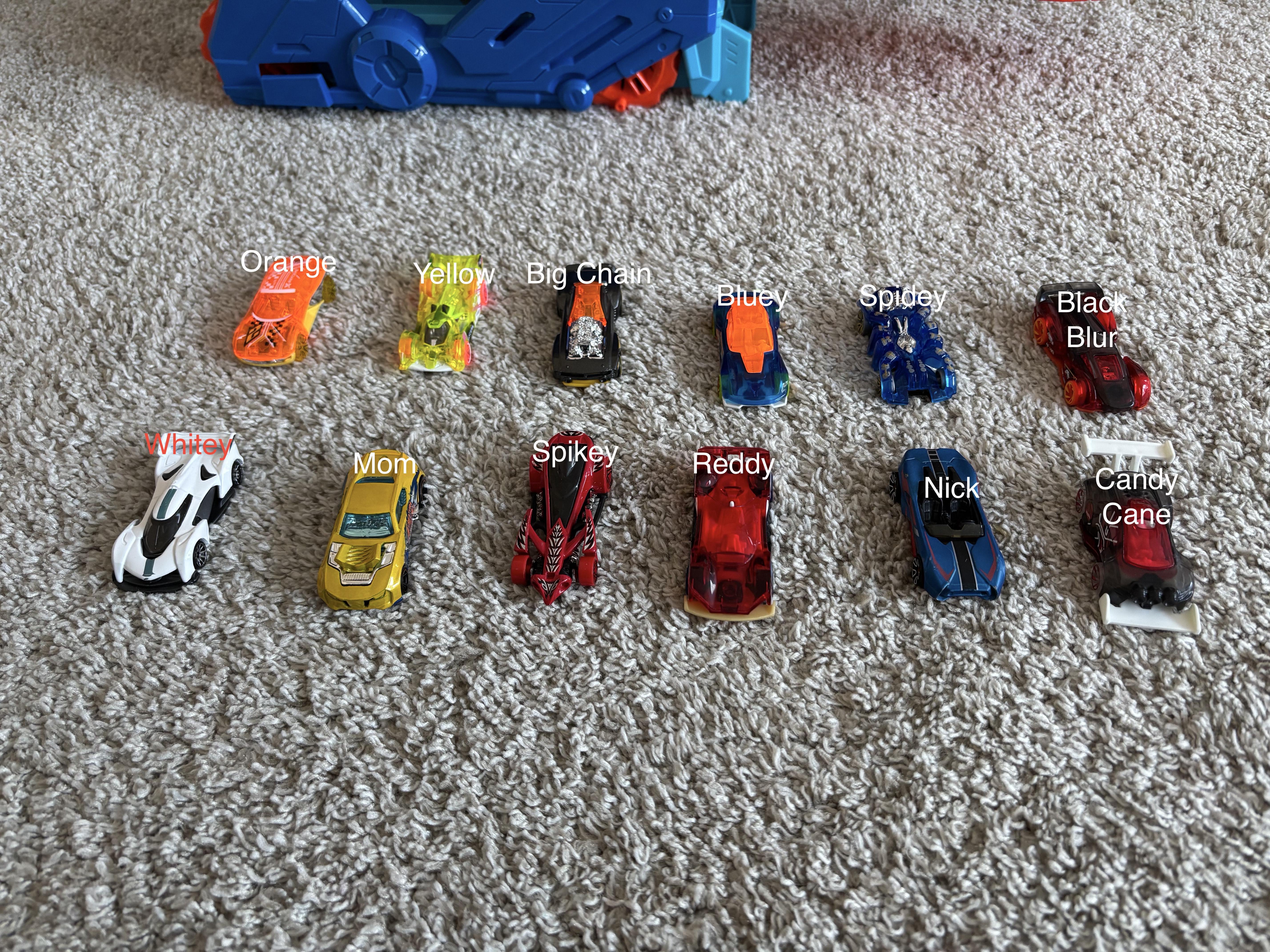
We had the patience to record 37 races (not bad!). That said, let's get into it.
 import sys
 import pandas as pd
 import numpy as np
 from matplotlib import pyplot as plt
 from pandas.plotting import register_matplotlib_converters
 from matplotlib.ticker import FuncFormatter
 import matplotlib.ticker as mtick
 register_matplotlib_converters()

 pct_formatter = FuncFormatter(lambda prop, _: "{:.1%}".format(prop))
 params = {"ytick.color" : "k",
           "xtick.color" : "k",
           "axes.labelcolor" : "k",
           "axes.edgecolor" : "k",
           "figure.figsize": (10,6),
           "axes.facecolor": [0.9, 0.9, 0.9],
           "axes.grid": True,
           "axes.labelsize": 10,
           "axes.titlesize": 10,
           "xtick.labelsize": 8,
           "ytick.labelsize": 8,
           "legend.fontsize": 8,
           "legend.facecolor": "w"}

 %matplotlib inline
 plt.rcParams.update(params)

 # helper funcs
 def getData():
     return (pd.read_csv('./data/HotWheels.csv')
             .assign(Winner=lambda x: x['Winner'] - 1)
             )

 def removeLaneCoding(tmp, num):
     return (tmp[[f'Lane{num}', 'Winner']]
             .assign(won=lambda x: x['Winner'] == (num-1))
             .rename(columns={f'Lane{num}': 'racer'})
             .drop(columns=['Winner'])
             )

 def explodeRows():
     tmp = getData()
     tmp = pd.concat([
         removeLaneCoding(tmp, 1),
         removeLaneCoding(tmp, 2)
     ])
     return tmp
Here's a quick look at the data. I originally encoded the car in lane 1, the car in lane 2, and which lane won. I updated the final column to whether lane2 won which will make modeling a little easier.
 df = getData()
 print(len(df))
 df.head()
37
| Lane1 | Lane2 | Winner | |
|---|---|---|---|
| 0 | Spikey | Mom | 1 |
| 1 | Whitey | Orange | 1 |
| 2 | BlackBlur | CandyCane | 0 |
| 3 | Reddy | Nick | 0 |
| 4 | Yellow | Spidey | 1 |
One of my first questions is which lane is faster. Lane2 won 21 of 37 races (57%). Hard to draw too much of a conclusion here though because I made no attempt to counterbalance cars across the lanes.
 (getData()
  .assign(_=lambda x: 'Lane2')
  .groupby('_')
  .agg({'Winner': ['sum', 'count', 'mean']})
  .reset_index()
  )
| _ | Winner | |||
|---|---|---|---|---|
| sum | count | mean | ||
| 0 | Lane2 | 21 | 37 | 0.567568 |
A natural next question is to look at the performance of the individual cars. To do this, I need to transform the data such that each race is two rows representing the outcome from each car's perspective.
 df = explodeRows()
 print(len(df))
 df.head()
74
| racer | won | |
|---|---|---|
| 0 | Spikey | False |
| 1 | Whitey | False |
| 2 | BlackBlur | True |
| 3 | Reddy | True |
| 4 | Yellow | False |
Now to group by car at look at the number of races, number of wins, and proportion of wins.
 (explodeRows()
  .groupby('racer')
  .agg({'won': ['sum', 'count', 'mean']})
  .reset_index()
  .sort_values('racer')
  )
| racer | won | |||
|---|---|---|---|---|
| sum | count | mean | ||
| 0 | BigChain | 4 | 5 | 0.800000 |
| 1 | BlackBlur | 5 | 8 | 0.625000 |
| 2 | Bluey | 6 | 9 | 0.666667 |
| 3 | CandyCane | 5 | 15 | 0.333333 |
| 4 | Mom | 3 | 4 | 0.750000 |
| 5 | Nick | 3 | 7 | 0.428571 |
| 6 | Orange | 7 | 10 | 0.700000 |
| 7 | Reddy | 1 | 3 | 0.333333 |
| 8 | Spidey | 2 | 4 | 0.500000 |
| 9 | Spikey | 0 | 2 | 0.000000 |
| 10 | Whitey | 0 | 2 | 0.000000 |
| 11 | Yellow | 1 | 5 | 0.200000 |
To create the model, I need to numerically encode the cars' identities. The only tricky thing here is not all cars have raced in both lanes.
 df = getData()
 racer_set = set(df['Lane1'].tolist() + df['Lane2'].tolist())
 racers = {x: i for i, x in enumerate(racer_set)}
 lane1_idx = np.array(df['Lane1'].map(racers))
 lane2_idx = np.array(df['Lane2'].map(racers))
 coords = {'racer': racers}
 print(coords)
{'racer': {'Whitey': 0, 'Yellow': 1, 'Bluey': 2, 'BigChain': 3, 'CandyCane': 4, 'Spidey': 5, 'Nick': 6, 'Spikey': 7, 'Mom': 8, 'Orange': 9, 'BlackBlur': 10, 'Reddy': 11}}
Now to design a model. The outcome is whether lane 2 won the race. The inputs are an intercept term (which I name lane2) and the quality of the two cars in the race. I figured these cars would be compared by subtracting one from another. I think this makes more sense than something like a ratio.....but feel free to let me know if you think otherwise.
 import pymc as pm
 import arviz as az

 with pm.Model(coords=coords) as model:
     # global model parameters
     lane2 = pm.Normal('lane2', mu=0, sigma=2)
     sd_racer = pm.HalfNormal('sd_racer', sigma=1)

     # team-specific model parameters
     mu_racers = pm.Normal('mu_racer', mu=0, sigma=sd_racer, dims='racer')

     # model
     μ = lane2 + mu_racers[lane2_idx] - mu_racers[lane1_idx]
     θ = pm.math.sigmoid(μ)
     yl = pm.Bernoulli('yl', p=θ, observed=df['Winner'])
     trace = pm.sample(2000, chains=4)

 az.plot_trace(trace, var_names=["lane2"], compact=False);
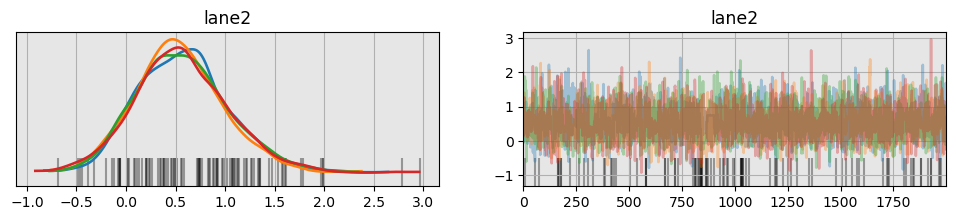
az.summary(trace, kind="diagnostics")
Onto results. First, is lane 2 faster. Here's a table with of lane2's (the intercept's) posterior.
 (az.hdi(trace)["lane2"]
  .sel({"hdi": ["lower", "higher"]})
  .to_dataframe()
  .reset_index()
  .assign(_='lane2')
  .pivot(index='_', columns='hdi', values='lane2')
  .reset_index()
  .assign(median=trace.posterior["lane2"].median(dim=("chain", "draw")).to_numpy())
  .assign(width=lambda x: x['higher'] - x['lower'])
  [['lower', 'median', 'higher', 'width']]
  )
| hdi | lower | median | higher | width |
|---|---|---|---|---|
| 0 | -0.292225 | 0.546044 | 1.481515 | 1.77374 |
Let's look at the portion of the intercept's posterior that is greater than 0. The model is 90% sure that lane 2 is faster.
 (trace
  .posterior["lane2"]
  .to_dataframe()
  .reset_index()
  .assign(greater_0=lambda x: x['lane2'] > 0)['greater_0'].mean()
  )
0.899875
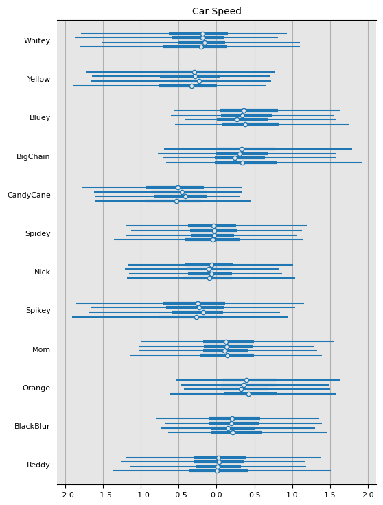
Next, onto the measurement of the cars. Candy Cane is my 3yr olds favorite so lots of trials there. It also pretty consistently loses. The model picks up on this. Not surprised to see Orange near the top. Big Chain also seems quite fast. I was not aware of how well Bluey was performing.
I'm not sure how to measure this (maybe it's the widthe of hdi interval) but I'm curious which cars I'd learn the most about given 1 additional race.
 (az.hdi(trace)["mu_racer"]
  .sel({"hdi": ["lower", "higher"]})
  .to_dataframe()
  .reset_index()
  .pivot(index='racer', columns='hdi', values='mu_racer')
  .reset_index()
  .merge(trace.posterior["mu_racer"].median(dim=("chain", "draw")).to_dataframe('median'),
         on='racer',
         how='left')
  .sort_values(by='median')
  .assign(width=lambda x: x['higher'] - x['lower'])
  [['racer', 'lower', 'median', 'higher', 'width']]
  )
| racer | lower | median | higher | width | |
|---|---|---|---|---|---|
| 3 | CandyCane | -1.630189 | -0.477509 | 0.385684 | 2.015874 |
| 11 | Yellow | -1.732217 | -0.281237 | 0.735534 | 2.467751 |
| 9 | Spikey | -1.861409 | -0.230835 | 0.939880 | 2.801289 |
| 10 | Whitey | -1.798544 | -0.181691 | 0.958850 | 2.757394 |
| 5 | Nick | -1.182705 | -0.082876 | 0.941209 | 2.123914 |
| 8 | Spidey | -1.248341 | -0.037978 | 1.116357 | 2.364698 |
| 7 | Reddy | -1.215164 | 0.021394 | 1.376155 | 2.591319 |
| 4 | Mom | -1.041651 | 0.127130 | 1.415593 | 2.457243 |
| 1 | BlackBlur | -0.747250 | 0.189628 | 1.351777 | 2.099027 |
| 0 | BigChain | -0.742637 | 0.298039 | 1.720762 | 2.463398 |
| 2 | Bluey | -0.606904 | 0.338542 | 1.570626 | 2.177530 |
| 6 | Orange | -0.519564 | 0.375396 | 1.543926 | 2.063490 |
Next I wanted to get a feel for how the cars compared in terms of how often I expect one car to win against another. I compared this by looking at the share of a car's posterior (racer_x) that was greater than the median of each other car's posterior (racer_y).
Only 2% of Candy Cane's posterior is greater than Orange's median!
 results = trace.posterior["mu_racer"].to_dataframe().reset_index()
 means = results.groupby('racer')['mu_racer'].median().reset_index()
 comparisons = (results
                .assign(key=0)
                .merge(means.assign(key=0), on='key', how='inner')
                .drop(columns='key')
                .assign(racerx_win_prob=lambda x: x['mu_racer_x'] > x['mu_racer_y'])
                .groupby(['racer_x', 'racer_y'])['racerx_win_prob']
                .mean()
                .reset_index()
                )
 (comparisons
  .pivot(index='racer_x', columns='racer_y', values='racerx_win_prob')
  )
| racery | BigChain | BlackBlur | Bluey | CandyCane | Mom | Nick | Orange | Reddy | Spidey | Spikey | Whitey | Yellow |
|---|---|---|---|---|---|---|---|---|---|---|---|---|
| racerx | ||||||||||||
| BigChain | 0.499875 | 0.581875 | 0.472875 | 0.952750 | 0.631125 | 0.803625 | 0.446500 | 0.714750 | 0.768125 | 0.888375 | 0.866375 | 0.908000 |
| BlackBlur | 0.415125 | 0.500000 | 0.388125 | 0.936250 | 0.555625 | 0.749125 | 0.359500 | 0.660375 | 0.711875 | 0.847125 | 0.819625 | 0.872375 |
| Bluey | 0.529875 | 0.628000 | 0.500000 | 0.970000 | 0.674250 | 0.840500 | 0.470500 | 0.763625 | 0.808125 | 0.913375 | 0.892625 | 0.930125 |
| CandyCane | 0.028625 | 0.052250 | 0.023000 | 0.500000 | 0.070875 | 0.193000 | 0.019250 | 0.122000 | 0.157750 | 0.313250 | 0.275625 | 0.355000 |
| Mom | 0.355750 | 0.445250 | 0.329125 | 0.883625 | 0.500000 | 0.669250 | 0.303750 | 0.585000 | 0.630875 | 0.779250 | 0.749625 | 0.807500 |
| Nick | 0.184750 | 0.257625 | 0.165375 | 0.790625 | 0.308625 | 0.500000 | 0.148625 | 0.397375 | 0.458500 | 0.633000 | 0.585500 | 0.670375 |
| Orange | 0.559625 | 0.652250 | 0.529375 | 0.979875 | 0.708500 | 0.856250 | 0.500000 | 0.786000 | 0.824625 | 0.927875 | 0.906625 | 0.943250 |
| Reddy | 0.289250 | 0.361250 | 0.265875 | 0.832625 | 0.406000 | 0.588250 | 0.247750 | 0.500000 | 0.549625 | 0.704125 | 0.665750 | 0.735625 |
| Spidey | 0.228875 | 0.297000 | 0.205625 | 0.806250 | 0.347250 | 0.543000 | 0.189500 | 0.442125 | 0.500000 | 0.664750 | 0.624750 | 0.696875 |
| Spikey | 0.131750 | 0.190250 | 0.116875 | 0.653750 | 0.226000 | 0.380875 | 0.104375 | 0.300375 | 0.344625 | 0.500000 | 0.465625 | 0.539500 |
| Whitey | 0.161500 | 0.208625 | 0.144375 | 0.693625 | 0.246875 | 0.418750 | 0.133125 | 0.332250 | 0.379125 | 0.538500 | 0.500000 | 0.572250 |
| Yellow | 0.095625 | 0.142375 | 0.083375 | 0.624250 | 0.176000 | 0.340250 | 0.073125 | 0.246250 | 0.300000 | 0.462000 | 0.426375 | 0.500000 |
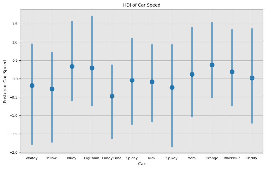
I visually depict each car's posterior in the next two plots. Not much sticks out to be beyond... I have some more playing to do!
 _, ax = plt.subplots()

 trace_hdi = az.hdi(trace)
 ax.scatter(racers.values(), trace.posterior["mu_racer"].median(dim=("chain", "draw")), color="C0", alpha=1, s=100)
 ax.vlines(
     racers.values(),
     trace_hdi["mu_racer"].sel({"hdi": "lower"}),
     trace_hdi["mu_racer"].sel({"hdi": "higher"}),
     alpha=0.6,
     lw=5,
     color="C0",
 )
 ax.set_xticks(list(racers.values()), racers.keys())
 ax.set_xlabel("Car")
 ax.set_ylabel("Posterior Car Speed")
 ax.set_title("HDI of Car Speed");
 class TeamLabeller(az.labels.BaseLabeller):
     def make_label_flat(self, var_name, sel, isel):
         sel_str = self.sel_to_str(sel, isel)
         return sel_str
 ax = az.plot_forest(trace, var_names=["mu_racer"], labeller=TeamLabeller())
 ax[0].set_title("Car Speed");