If you're just finding this post, please check out Erik Marsja's post describing the same functionality in well-maintained python software that wasn't available when I originally wrote this post.
I love doing data analyses with pandas, numpy, sci-py etc., but I often need to run repeated measures ANOVAs, which are not implemented in any major python libraries. Python Psychologist shows how to do repeated measures ANOVAs yourself in python, but I find using a widley distributed implementation comforting...
In this post I show how to execute a repeated measures ANOVAs using the rpy2 library, which allows us to move data between python and R, and execute R commands from python. I use rpy2 to load the car library and run the ANOVA.
I will show how to run a one-way repeated measures ANOVA and a two-way repeated measures ANOVA.
 #first import the libraries I always use.
 import numpy as np, scipy.stats, pandas as pd

 import matplotlib as mpl
 import matplotlib.pyplot as plt
 import pylab as pl
 %matplotlib inline
 pd.options.display.mpl_style = 'default'
 plt.style.use('ggplot')
 mpl.rcParams['font.family'] = ['Bitstream Vera Sans']
Below I use the random library to generate some fake data. I seed the random number generator with a one so that this analysis can be replicated.
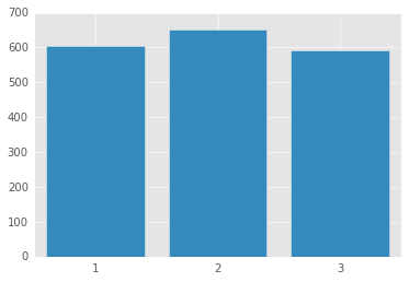
I will generated 3 conditions which represent 3 levels of a single variable.
The data are generated from a gaussian distribution. The second condition has a higher mean than the other two conditions.
 import random

 random.seed(1) #seed random number generator
 cond_1 = [random.gauss(600,30) for x in range(30)] #condition 1 has a mean of 600 and standard deviation of 30
 cond_2 = [random.gauss(650,30) for x in range(30)] #u=650 and sd=30
 cond_3 = [random.gauss(600,30) for x in range(30)] #u=600 and sd=30

 plt.bar(np.arange(1,4),[np.mean(cond_1),np.mean(cond_2),np.mean(cond_3)],align='center') #plot data
 plt.xticks([1,2,3]);
Next, I load rpy2 for ipython. I am doing these analyses with ipython in a jupyter notebook (highly recommended).
%load_ext rpy2.ipython
Here's how to run the ANOVA. Note that this is a one-way anova with 3 levels of the factor.
 #pop the data into R
 %Rpush cond_1 cond_2 cond_3

 #label the conditions
 %R Factor <- c('Cond1','Cond2','Cond3')
 #create a vector of conditions
 %R idata <- data.frame(Factor)

 #combine data into single matrix
 %R Bind <- cbind(cond_1,cond_2,cond_3)
 #generate linear model
 %R model <- lm(Bind~1)

 #load the car library. note this library must be installed.
 %R library(car)
 #run anova
 %R analysis <- Anova(model,idata=idata,idesign=~Factor,type="III")
 #create anova summary table
 %R anova_sum = summary(analysis)

 #move the data from R to python
 %Rpull anova_sum
 print anova_sum


Type III Repeated Measures MANOVA Tests:

------------------------------------------

Term: (Intercept)

 Response transformation matrix:
       (Intercept)
cond_1           1
cond_2           1
cond_3           1

Sum of squares and products for the hypothesis:
            (Intercept)
(Intercept)   102473990

Sum of squares and products for error:
            (Intercept)
(Intercept)     78712.7

Multivariate Tests: (Intercept)
                 Df test stat approx F num Df den Df     Pr(>F)
Pillai            1    0.9992 37754.33      1     29 < 2.22e-16 ***
Wilks             1    0.0008 37754.33      1     29 < 2.22e-16 ***
Hotelling-Lawley  1 1301.8736 37754.33      1     29 < 2.22e-16 ***
Roy               1 1301.8736 37754.33      1     29 < 2.22e-16 ***
---
Signif. codes:  0 ‘***’ 0.001 ‘**’ 0.01 ‘*’ 0.05 ‘.’ 0.1 ‘ ’ 1

------------------------------------------

Term: Factor

 Response transformation matrix:
       Factor1 Factor2
cond_1       1       0
cond_2       0       1
cond_3      -1      -1

Sum of squares and products for the hypothesis:
          Factor1   Factor2
Factor1  3679.584  19750.87
Factor2 19750.870 106016.58

Sum of squares and products for error:
         Factor1  Factor2
Factor1 40463.19 27139.59
Factor2 27139.59 51733.12

Multivariate Tests: Factor
                 Df test stat approx F num Df den Df    Pr(>F)
Pillai            1 0.7152596 35.16759      2     28 2.303e-08 ***
Wilks             1 0.2847404 35.16759      2     28 2.303e-08 ***
Hotelling-Lawley  1 2.5119704 35.16759      2     28 2.303e-08 ***
Roy               1 2.5119704 35.16759      2     28 2.303e-08 ***
---
Signif. codes:  0 ‘***’ 0.001 ‘**’ 0.01 ‘*’ 0.05 ‘.’ 0.1 ‘ ’ 1

Univariate Type III Repeated-Measures ANOVA Assuming Sphericity

                  SS num Df Error SS den Df         F    Pr(>F)
(Intercept) 34157997      1    26238     29 37754.334 < 2.2e-16 ***
Factor         59964      2    43371     58    40.094 1.163e-11 ***
---
Signif. codes:  0 ‘***’ 0.001 ‘**’ 0.01 ‘*’ 0.05 ‘.’ 0.1 ‘ ’ 1


Mauchly Tests for Sphericity

       Test statistic p-value
Factor        0.96168 0.57866


Greenhouse-Geisser and Huynh-Feldt Corrections
 for Departure from Sphericity

        GG eps Pr(>F[GG])
Factor 0.96309  2.595e-11 ***
---
Signif. codes:  0 ‘***’ 0.001 ‘**’ 0.01 ‘*’ 0.05 ‘.’ 0.1 ‘ ’ 1

        HF eps   Pr(>F[HF])
Factor 1.03025 1.163294e-11
The ANOVA table isn't pretty, but it works. As you can see, the ANOVA was wildly significant.
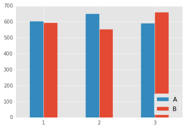
Next, I generate data for a two-way (2x3) repeated measures ANOVA. Condition A is the same data as above. Condition B has a different pattern (2 is lower than 1 and 3), which should produce an interaction.
 random.seed(1)

 cond_1a = [random.gauss(600,30) for x in range(30)] #u=600,sd=30
 cond_2a = [random.gauss(650,30) for x in range(30)] #u=650,sd=30
 cond_3a = [random.gauss(600,30) for x in range(30)] #u=600,sd=30

 cond_1b = [random.gauss(600,30) for x in range(30)] #u=600,sd=30
 cond_2b = [random.gauss(550,30) for x in range(30)] #u=550,sd=30
 cond_3b = [random.gauss(650,30) for x in range(30)] #u=650,sd=30

 width = 0.25
 plt.bar(np.arange(1,4)-width,[np.mean(cond_1a),np.mean(cond_2a),np.mean(cond_3a)],width)
 plt.bar(np.arange(1,4),[np.mean(cond_1b),np.mean(cond_2b),np.mean(cond_3b)],width,color=plt.rcParams['axes.color_cycle'][0])
 plt.legend(['A','B'],loc=4)
 plt.xticks([1,2,3]);
 %Rpush cond_1a cond_1b cond_2a cond_2b cond_3a cond_3b

 %R Factor1 <- c('A','A','A','B','B','B')
 %R Factor2 <- c('Cond1','Cond2','Cond3','Cond1','Cond2','Cond3')
 %R idata <- data.frame(Factor1, Factor2)

 #make sure the vectors appear in the same order as they appear in the dataframe
 %R Bind <- cbind(cond_1a, cond_2a, cond_3a, cond_1b, cond_2b, cond_3b)
 %R model <- lm(Bind~1)

 %R library(car)
 %R analysis <- Anova(model, idata=idata, idesign=~Factor1*Factor2, type="III")
 %R anova_sum = summary(analysis)
 %Rpull anova_sum

 print anova_sum


Type III Repeated Measures MANOVA Tests:

------------------------------------------

Term: (Intercept)

 Response transformation matrix:
        (Intercept)
cond_1a           1
cond_2a           1
cond_3a           1
cond_1b           1
cond_2b           1
cond_3b           1

Sum of squares and products for the hypothesis:
            (Intercept)
(Intercept)   401981075

Sum of squares and products for error:
            (Intercept)
(Intercept)    185650.5

Multivariate Tests: (Intercept)
                 Df test stat approx F num Df den Df     Pr(>F)
Pillai            1    0.9995 62792.47      1     29 < 2.22e-16 ***
Wilks             1    0.0005 62792.47      1     29 < 2.22e-16 ***
Hotelling-Lawley  1 2165.2575 62792.47      1     29 < 2.22e-16 ***
Roy               1 2165.2575 62792.47      1     29 < 2.22e-16 ***
---
Signif. codes:  0 ‘***’ 0.001 ‘**’ 0.01 ‘*’ 0.05 ‘.’ 0.1 ‘ ’ 1

------------------------------------------

Term: Factor1

 Response transformation matrix:
        Factor11
cond_1a        1
cond_2a        1
cond_3a        1
cond_1b       -1
cond_2b       -1
cond_3b       -1

Sum of squares and products for the hypothesis:
         Factor11
Factor11 38581.51

Sum of squares and products for error:
         Factor11
Factor11 142762.3

Multivariate Tests: Factor1
                 Df test stat approx F num Df den Df    Pr(>F)
Pillai            1 0.2127533 7.837247      1     29 0.0090091 **
Wilks             1 0.7872467 7.837247      1     29 0.0090091 **
Hotelling-Lawley  1 0.2702499 7.837247      1     29 0.0090091 **
Roy               1 0.2702499 7.837247      1     29 0.0090091 **
---
Signif. codes:  0 ‘***’ 0.001 ‘**’ 0.01 ‘*’ 0.05 ‘.’ 0.1 ‘ ’ 1

------------------------------------------

Term: Factor2

 Response transformation matrix:
        Factor21 Factor22
cond_1a        1        0
cond_2a        0        1
cond_3a       -1       -1
cond_1b        1        0
cond_2b        0        1
cond_3b       -1       -1

Sum of squares and products for the hypothesis:
         Factor21 Factor22
Factor21 91480.01 77568.78
Factor22 77568.78 65773.02

Sum of squares and products for error:
         Factor21 Factor22
Factor21 90374.60 56539.06
Factor22 56539.06 87589.85

Multivariate Tests: Factor2
                 Df test stat approx F num Df den Df    Pr(>F)
Pillai            1 0.5235423 15.38351      2     28 3.107e-05 ***
Wilks             1 0.4764577 15.38351      2     28 3.107e-05 ***
Hotelling-Lawley  1 1.0988223 15.38351      2     28 3.107e-05 ***
Roy               1 1.0988223 15.38351      2     28 3.107e-05 ***
---
Signif. codes:  0 ‘***’ 0.001 ‘**’ 0.01 ‘*’ 0.05 ‘.’ 0.1 ‘ ’ 1

------------------------------------------

Term: Factor1:Factor2

 Response transformation matrix:
        Factor11:Factor21 Factor11:Factor22
cond_1a                 1                 0
cond_2a                 0                 1
cond_3a                -1                -1
cond_1b                -1                 0
cond_2b                 0                -1
cond_3b                 1                 1

Sum of squares and products for the hypothesis:
                  Factor11:Factor21 Factor11:Factor22
Factor11:Factor21          179585.9            384647
Factor11:Factor22          384647.0            823858

Sum of squares and products for error:
                  Factor11:Factor21 Factor11:Factor22
Factor11:Factor21          92445.33          45639.49
Factor11:Factor22          45639.49          89940.37

Multivariate Tests: Factor1:Factor2
                 Df test stat approx F num Df den Df     Pr(>F)
Pillai            1  0.901764 128.5145      2     28 7.7941e-15 ***
Wilks             1  0.098236 128.5145      2     28 7.7941e-15 ***
Hotelling-Lawley  1  9.179605 128.5145      2     28 7.7941e-15 ***
Roy               1  9.179605 128.5145      2     28 7.7941e-15 ***
---
Signif. codes:  0 ‘***’ 0.001 ‘**’ 0.01 ‘*’ 0.05 ‘.’ 0.1 ‘ ’ 1

Univariate Type III Repeated-Measures ANOVA Assuming Sphericity

                      SS num Df Error SS den Df          F    Pr(>F)
(Intercept)     66996846      1    30942     29 62792.4662 < 2.2e-16 ***
Factor1             6430      1    23794     29     7.8372  0.009009 **
Factor2            26561      2    40475     58    19.0310  4.42e-07 ***
Factor1:Factor2   206266      2    45582     58   131.2293 < 2.2e-16 ***
---
Signif. codes:  0 ‘***’ 0.001 ‘**’ 0.01 ‘*’ 0.05 ‘.’ 0.1 ‘ ’ 1


Mauchly Tests for Sphericity

                Test statistic p-value
Factor2                0.96023 0.56654
Factor1:Factor2        0.99975 0.99648


Greenhouse-Geisser and Huynh-Feldt Corrections
 for Departure from Sphericity

                 GG eps Pr(>F[GG])
Factor2         0.96175  6.876e-07 ***
Factor1:Factor2 0.99975  < 2.2e-16 ***
---
Signif. codes:  0 ‘***’ 0.001 ‘**’ 0.01 ‘*’ 0.05 ‘.’ 0.1 ‘ ’ 1

                  HF eps   Pr(>F[HF])
Factor2         1.028657 4.420005e-07
Factor1:Factor2 1.073774 2.965002e-22
Again, the anova table isn't too pretty.
This obviously isn't the most exciting post in the world, but its a nice bit of code to have in your back pocket if you're doing experimental analyses in python.