In a previous post, I described how to download and clean data for understanding how likely a baseball player is to hit into an error given that they hit the ball into play.

This analysis will statistically demonstrate that some players are more likely to hit into errors than others.

Errors are uncommon, so players hit into errors very infrequently. Estimating the likelihood of an infrequent event is hard and requires lots of data. To acquire as much data as possible, I wrote a bash script that will download data for all players between 1970 and 2018.

This data enables me to use data from multiple years for each player, giving me more data when estimating how likely a particular player is to hit into an error.

1
2
3
4
5
6
7
8
9
10
11
12

%%bash

for i in {1970..2018}; do
    echo "YEAR: $i"
    ../scripts/get_data.sh ${i};
done

find processed_data/* -type f -name 'errors_bip.out' | \
    xargs awk '{print $0", "FILENAME}' | \
    sed s1processed_data/11g1 | \
    sed s1/errors_bip.out11g1 > \
        processed_data/all_errors_bip.out

The data has 5 columns: playerid, playername, errors hit into, balls hit into play (BIP), and year. The file does not have a header.

1
2

%%bash
head ../processed_data/all_errors_bip.out

aaroh101, Hank Aaron, 8, 453, 1970
aarot101, Tommie Aaron, 0, 53, 1970
abert101, Ted Abernathy, 0, 10, 1970
adaij101, Jerry Adair, 0, 24, 1970
ageet101, Tommie Agee, 12, 480, 1970
akerj102, Jack Aker, 0, 10, 1970
alcal101, Luis Alcaraz, 1, 107, 1970
alleb105, Bernie Allen, 1, 240, 1970
alled101, Dick Allen, 4, 341, 1970
alleg101, Gene Alley, 6, 356, 1970

I can load the data into pandas using the following command.

1
2
3
4
5

import pandas as pd

DF = pd.read_csv('../processed_data/all_errors_bip.out',
                 header=None,
                 names=['playerid', 'player_name', 'errors', 'bip', 'year'])

1

DF.head()

1

len(DF)

38870

I have almost 39,000 year, player combinations…. a good amount of data to play with.

While exploring the data, I noticed that players hit into errors less frequently now than they used to. Let’s see how the probability that a player hits into an error has changed across the years.

1
2
3
4
5
6
7
8
9
10
11
12

%matplotlib inline

YEAR_DF = (DF
           .groupby("year")
           .agg({
               "errors": "sum",
               "bip": "sum"
           })
           .assign(prop_error=lambda x: x["errors"] / x["bip"])
          )

YEAR_DF["prop_error"].plot(style="o-");

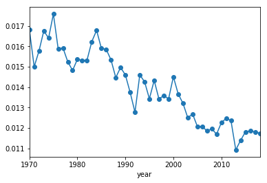
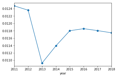
Interestingly, the proportion of errors per BIP has been dropping over time. I am not sure if this is a conscious effort by MLB score keepers, a change in how hitters hit, or improved fielding (but I suspect it’s the score keepers). It looks like this drop in errors per BIP leveled off around 2015. Zooming in.

1

YEAR_DF[YEAR_DF.index > 2010]["prop_error"].plot(style="o-");

I explore this statistically in a jupyter notebook on my github.

Because I don’t want year to confound the analysis, I remove all data before 2015.

1

DF = DF[DF["year"] >= 2015]

1

len(DF)

3591

This leaves me with 3500 year, player combinations.

Next I combine players’ data across years.

1

GROUPED_DF = DF.groupby(["playerid", "player_name"]).agg({"errors": "sum", "bip": "sum"}).reset_index()

1

GROUPED_DF.describe()

I want an idea for how likely players are to hit into errors.

1
2
3

TOTALS = GROUPED_DF.agg({"errors": "sum", "bip": "sum"})
ERROR_RATE = TOTALS["errors"] / TOTALS["bip"]
ERROR_RATE

0.011801960251664112

Again, errors are very rare, so I want know how many “trials” (BIP) I need for a reasonable estimate of how likely each player is to hit into an error.

I’d like the majority of players to have at least 5 errors. I can estimate how many BIP that would require.

1

5. /ERROR_RATE

423.65843413978496

Looks like I should require at least 425 BIP for each player. I round this to 500.

1

GROUPED_DF = GROUPED_DF[GROUPED_DF["bip"] > 500]

1

GROUPED_DF = GROUPED_DF.reset_index(drop=True)

1

GROUPED_DF.head()

1

GROUPED_DF.describe()

I’ve identified 354 players who have enough BIP for me to estimate how frequently they hit into errors.

Below, I plot how the likelihood of hitting into errors is distributed.

1
2
3
4

%matplotlib inline

GROUPED_DF["prop_error"] = GROUPED_DF["errors"] / GROUPED_DF["bip"]
GROUPED_DF["prop_error"].hist();

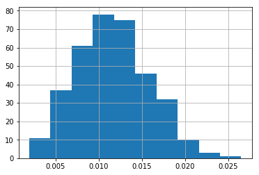
The question is whether someone who has hit into errors in 2% of their BIP is more likely to hit into an error than someone who has hit into errors in 0.5% of their BIP (or is this all just random variation).

To try and estimate this, I treat each BIP as a Bernoulli trial. Hitting into an error is a “success”. I use a Binomial distribution to model the number of “successes”. I would like to know if different players are more or less likely to hit into errors. To do this, I model each player as having their own Binomial distribution and ask whether p (the probability of success) differs across players.

To answer this question, I could use a chi square contingency test but this would only tell me whether players differ at all and not which players differ.

The traditional way to identify which players differ is to do pairwise comparisons, but this would result in TONS of comparisons making false positives all but certain.

Another option is to harness Bayesian statistics and build a Hierarchical Beta-Binomial model. The intuition is that each player’s probability of hitting into an error is drawn from a Beta distribution. I want to know whether these Beta distributions are different. I then assume I can best estimate a player’s Beta distribution by using that particular player’s data AND data from all players together.

The model is built so that as I accrue data about a particular player, I will trust that data more and more, relying less and less on data from all players. This is called partial pooling. Here’s a useful explanation.

I largely based my analysis on this tutorial. Reference the tutorial for an explanation of how I choose my priors. I ended up using a greater lambda value (because the model sampled better) in the Exponential prior, and while this did lead to more extreme estimates of error likelihood, it didn’t change the basic story.

1
2
3
4
5
6
7
8
9
10
11
12
13
14
15
16
17
18

import pymc3 as pm
import numpy as np
import theano.tensor as tt

with pm.Model() as model:

    phi = pm.Uniform('phi', lower=0.0, upper=1.0)

    kappa_log = pm.Exponential('kappa_log', lam=25.)
    kappa = pm.Deterministic('kappa', tt.exp(kappa_log))

    rates = pm.Beta('rates', alpha=phi*kappa, beta=(1.0-phi)*kappa, shape=len(GROUPED_DF))

    trials = np.array(GROUPED_DF["bip"])
    successes = np.array(GROUPED_DF["errors"])

    obs = pm.Binomial('observed_values', trials, rates, observed=successes)
    trace = pm.sample(2000, tune=1000, chains=2, cores=2, nuts_kwargs={'target_accept': .95})

Auto-assigning NUTS sampler...
Initializing NUTS using jitter+adapt_diag...
Multiprocess sampling (2 chains in 2 jobs)
NUTS: [rates, kappa_log, phi]
Sampling 2 chains: 100%|██████████| 6000/6000 [01:47<00:00, 28.06draws/s] 

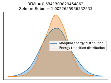
Check whether the model converged.

1

max(np.max(score) for score in pm.gelman_rubin(trace).values())

1.0022635936332533

1
2
3

bfmi = pm.bfmi(trace)
max_gr = max(np.max(gr_stats) for gr_stats in pm.gelman_rubin(trace).values())
(pm.energyplot(trace, figsize=(6, 4)).set_title("BFMI = {}\nGelman-Rubin = {}".format(bfmi, max_gr)));

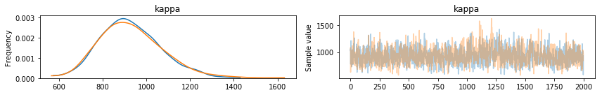
The most challenging parameter to fit is kappa which modulates for the variance in the likelihood to hit into an error. I take a look at it to make sure things look as expected.

1

pm.summary(trace, varnames=["kappa"])

1

pm.traceplot(trace, varnames=['kappa']);

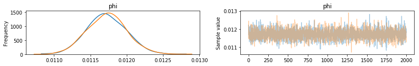
I can also look at phi, the estimated global likelihood to hit into an error.

1

pm.traceplot(trace, varnames=['phi']);

Finally, I can look at how all players vary in their likelihood to hit into an error.

1

pm.traceplot(trace, varnames=['rates']);

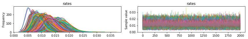
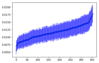
Obviously, the above plot is a lot to look at it, so let’s order players by how likely the model believes they are to hit in an error.

1
2
3
4
5
6
7
8
9
10
11
12
13
14
15
16

from matplotlib import pyplot as plt

rate_means = trace['rates', 1000:].mean(axis=0)
rate_se = trace['rates', 1000:].std(axis=0)

mean_se = [(x, y, i) for i, x, y in zip(GROUPED_DF.index, rate_means, rate_se)]
sorted_means_se = sorted(mean_se, key=lambda x: x[0])
sorted_means = [x[0] for x in sorted_means_se]
sorted_se = [x[1] for x in sorted_means_se]

x = np.arange(len(sorted_means))

plt.plot(x, sorted_means, 'o', alpha=0.25);

for x_val, m, se in zip(x, sorted_means, sorted_se):
    plt.plot([x_val, x_val], [m-se, m+se], 'b-', alpha=0.5)

Now, the ten players who are most likely to hit into an error.

1
2
3

estimated_mean = pm.summary(trace, varnames=["rates"]).iloc[[x[2] for x in sorted_means_se[-10:]]]["mean"]

GROUPED_DF.loc[[x[2] for x in sorted_means_se[-10:]], :].assign(estimated_mean=estimated_mean.values).iloc[::-1]

And the 10 players who are least likely to hit in an error.

1
2
3

estimated_mean = pm.summary(trace, varnames=["rates"]).iloc[[x[2] for x in sorted_means_se[:10]]]["mean"]

GROUPED_DF.loc[[x[2] for x in sorted_means_se[:10]], :].assign(estimated_mean=estimated_mean.values)

It looks to me like players who hit more ground balls are more likely to hit into an error than players who predominately hits fly balls and line-drives. This makes sense since infielders make more errors than outfielders.

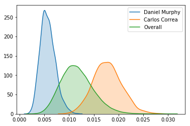
Using the posterior distribution of estimated likelihoods to hit into an error, I can assign a probability to whether Carlos Correa is more likely to hit into an error than Daniel Murphy.

1

np.mean(trace['rates', 1000:][:, 71] <= trace['rates', 1000:][:, 226])

0.0

The model believes Correa is much more likely to hit into an error than Murphy!

I can also plot these players’ posterior distributions.

1
2
3
4
5

import seaborn as sns

sns.kdeplot(trace['rates', 1000:][:, 226], shade=True, label="Daniel Murphy");
sns.kdeplot(trace['rates', 1000:][:, 71], shade=True, label="Carlos Correa");
sns.kdeplot(trace['rates', 1000:].flatten(), shade=True, label="Overall");

Finally, I can look exclusively at how the posterior distributions of the ten most likely and 10 least likely players to hit into an error compare.

1
2

sns.kdeplot(trace['rates', 1000:][:, [x[2] for x in sorted_means_se[-10:]]].flatten(), shade=True, label="10 Least Likely");
sns.kdeplot(trace['rates', 1000:][:, [x[2] for x in sorted_means_se[:10]]].flatten(), shade=True, label="10 Most Likely");

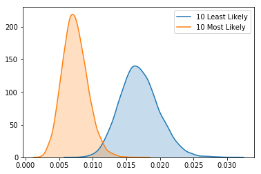
All in all, this analysis makes it obvious that some players are more likely to hit into errors than other players. This is probably driven by how often players hit ground balls.