Dan Vatterott

Data Scientist

Data Onboarding Checklist

I’m a checklist addict. While our team has a document on acquiring different accounts, reviewing our workflows, reviewing code repos etc., this document doesn’t provide any prioritization.

I created the following checklist (markdown) to give a condensed view of what a manager and new hire should accomplish by the end of the first week following a new hire’s start.

I wasn’t able to find existing onboarding checklists so I hope you find this useful!

1
2
3
4
5
6
7
8
9
10
11
12
13
14
15
16
17
18
19
20
21
22
23
24
25
26
27
28
29
30
31
32
33
34
35
36
37
38
39
40
41
42
43
44
45
46
47
48
49
50
51
52
53
54
55
56
57
58
59
60
61
62
63
64
65
66
67
# Request Email
  + [ ] Request an email account
# Request Equipment
  + [ ] Request Laptop
  + [ ] Request monitor, keyboard, & mouse
# Request Accounts
  + [ ] Request Cloud Account
  + [ ] Request Data Warehouse Account
  + [ ] Request Dashboarding Account
  + [ ] Request Version Control Account
  + [ ] Request Workflow Management Account
# Install Software
  + [ ] Text Editor / IDE
  + [ ] Code Packaging and Dependency Management Software
  + [ ] Office Suite
  + [ ] Communication Platforms (e.g., Zoom, Slack)
  + [ ] CLIs
  + [ ] Clone Repos
# Schedule Intro Meetings
  + [ ] Collaborator A
  + [ ] Team B
  + [ ] Etc.
# Add to Meetings/Channels/Distribution Lists
## Meetings
  + [ ] Daily Stand-up
  + [ ] Weekly 1on1
  + [ ] Weekly Larger Team Meeting
## Distribution Lists
  + [ ] Example A
## Communication Channels
  + [ ] Example A
# Templates
  + [ ] Presentations
  + [ ] Dashboards
  + [ ] Document Headers
  + [ ] Spreadsheets
# Data Schemas Intro
  + [ ] Schema X
  + [ ] Schema Y
# 7/30/60/90 Day Plans
## 7 Day
  + [ ] Set-Up Machine
  + [ ] Clone Repos
  + [ ] Run Repo Unit-Tests
  + [ ] Request Accounts and Software
  + [ ] Automation Intro
  + [ ] Cloud Services Intro
  + [ ] Data Warehouse Intro
  + [ ] Review Jargon
## 30 Day
  + [ ] Discuss Order of Code Repo Reviews
  + [ ] Discuss 30 Day Project
  + [ ] Discuss 30 Day Goals
## 60 Day
  + [ ] Discuss 60 Day Project
  + [ ] Discuss 60 Day Goals
## 90 Day
  + [ ] Discuss 90 Day Project
  + [ ] Discuss 90 Day Goals
# Communication/Work Style
  + [ ] Discuss Work Styles
  + [ ] Discuss Communication Styles
  + [ ] Discuss Preferred Feedback Style
  + [ ] Discuss Preferred Hours
  + [ ] Discuss a Vision of Success
# Jargon
  + [ ] Review Company/Business Jargon

Posting Collections as Hive Tables

I was recently asked to post a series of parquet collection as tables so analysts could query them in SQL. This should be straight forward, but it took me awhile to figure out. Hopefully, you find this post before spending too much time on such an easy task.

You should use the CREATE TABLE. This is pretty straight forward. By creating a permanent table (rather than a temp table), you can use a database name. Also, by using a table (rather than a view), you can load the data from an s3 location.

Next, you can specify the table’s schema. Again, this is pretty straight forward. Columns used to partition the data should be declared here.

Next, you can specify how the data is stored (below, I use Parquet) and how the data is partitioned (below, there are two partitioning columns).

Finally, you specify the data’s location.

The part that really threw me for a loop here is that I wasn’t done yet! You need one more command so that Spark can go examine the partitions - MSCK REPAIR TABLE. Also please note that this command needs to be re-run whenever a partition is added.

1
2
3
4
5
6
7
8
9
spark.sql("""
CREATE TABLE my_db.my_table (
(example_key INT, example_col STRING, example_string STRING, example_date STRING)
)
USING PARQUET
PARTITIONED BY (example_string, example_date)
LOCATION 's3://my.example.bucket/my_db/my_table/'
"""
spark.sql("MSCK REPAIR TABLE my_db.my_table")

Hope this post saves you some time!

Balancing Model Weights in PySpark

Imbalanced classes is a common problem. Scikit-learn provides an easy fix - “balancing” class weights. This makes models more likely to predict the less common classes (e.g., logistic regression).

The PySpark ML API doesn’t have this same functionality, so in this blog post, I describe how to balance class weights yourself.

1
2
3
4
5
6
7
8
9
10
11
import numpy as np
import pandas as pd
from itertools import chain
from pyspark.sql import SparkSession
from pyspark import SparkContext
from pyspark.sql import functions as F
from pyspark.ml.feature import VectorAssembler
from pyspark.ml.classification import LogisticRegression

sc = SparkContext("local", "Example")
spark = SparkSession(sc)

Generate some random data and put the data in a Spark DataFrame. Note that the input variables are not predictive. The model will behave randomly. This is okay, since I am not interested in model accuracy.

1
2
3
4
5
6
7
8
9
10
11
12
X = np.random.normal(0, 1, (10000, 10))

y = np.ones(X.shape[0]).astype(int)
y[:1000] = 0
np.random.shuffle(y)

print(np.mean(y)) # 0.9

X = np.append(X, y.reshape((10000, 1)), 1)

DF = spark.createDataFrame(pd.DataFrame(X))
DF = DF.withColumnRenamed("10", "y")

Here’s how Scikit-learn computes class weights when “balanced” weights are requested.

1
2
3
4
5
6
# class weight
# https://scikit-learn.org/stable/modules/generated/sklearn.linear_model.LogisticRegression.html
# n_samples / (n_classes * np.bincount(y)).

class_weights = {i: ii for i, ii in zip(np.unique(y), len(y) / (len(np.unique(y)) * np.bincount(y)))}
print(class_weights) # {0: 5.0, 1: 0.5555555555555556}

Here’s how we can compute “balanced” weights with data from a PySpark DataFrame.

1
2
3
4
5
6
7
8
y_collect = DF.select("y").groupBy("y").count().collect()
unique_y = [x["y"] for x in y_collect]
total_y = sum([x["count"] for x in y_collect])
unique_y_count = len(y_collect)
bin_count = [x["count"] for x in y_collect]

class_weights_spark = {i: ii for i, ii in zip(unique_y, total_y / (unique_y_count * np.array(bin_count)))}
print(class_weights_spark) # {0.0: 5.0, 1.0: 0.5555555555555556}

PySpark needs to have a weight assigned to each instance (i.e., row) in the training set. I create a mapping to apply a weight to each training instance.

1
2
3
mapping_expr = F.create_map([F.lit(x) for x in chain(*class_weights_spark.items())])

DF = DF.withColumn("weight", mapping_expr.getItem(F.col("y")))

I assemble all the input features into a vector.

1
2
3
assembler = VectorAssembler(inputCols=[str(x) for x in range(10)], outputCol="features")

DF = assembler.transform(DF).drop(*[str(x) for x in range(10)])

And train a logistic regression. Without the instance weights, the model predicts all instances as the frequent class.

1
2
3
lr = LogisticRegression(featuresCol="features", labelCol="y")
lrModel = lr.fit(DF)
lrModel.transform(DF).agg(F.mean("prediction")).show()
+---------------+
|avg(prediction)|
+---------------+
|            1.0|
+---------------+

With the weights, the model assigns half the instances to each class (even the less commmon one).

1
2
3
lr = LogisticRegression(featuresCol="features", labelCol="y", weightCol="weight")
lrModel = lr.fit(DF)
lrModel.transform(DF).agg(F.mean("prediction")).show()
+---------------+
|avg(prediction)|
+---------------+
|         0.5089|
+---------------+

Creating a CDF in PySpark

CDFs are a useful tool for understanding your data. This tutorial will demonstrate how to create a CDF in PySpark.

I start by creating normally distributed, fake data.

1
2
3
4
5
6
7
8
9
10
11
import numpy as np
from pyspark.sql import SparkSession
from pyspark import SparkContext
from pyspark.sql import functions as F
from pyspark.sql.window import Window

sc = SparkContext("local", "Example")
spark = SparkSession(sc)

a = (sc.parallelize([(float(x),) for x in np.random.normal(0, 1, 1000)]).toDF(['X']))
a.limit(5).show()
X
1.3162087724709406
-0.9226127327757598
0.5388249247619141
-0.38263792383896356
0.20584675505779562

To create the CDF I need to use a window function to order the data. I can then use percent_rank to retrieve the percentile associated with each value.

The only trick here is I round the column of interest to make sure I don’t retrieve too much data onto the master node (not a concern here, but always good to think about).

After rounding, I group by the variable of interest, again, to limit the amount of data returned.

1
2
3
4
5
6
7
8
9
win = Window.orderBy('X')

output = (a
          .withColumn('cumulative_probability', F.percent_rank().over(win))
          .withColumn("X", F.round(F.col("X"), 1))
          .groupBy("X")
          .agg(F.max("cumulative_probability").alias("cumulative_probability"),F.count('*').alias("my_count")))

output.limit(5).show()
X cumulative_probability my_count
-3.5 0.0 1
-3.3 0.001001001001001001 1
-2.9 0.002002002002002002 1
-2.8 0.003003003003003003 1
-2.7 0.004004004004004004 1

A CDF should report the percent of data less than or equal to the specified value. The data returned above is the percent of data less than the specified value. We need to fix this by shifting the data up.

To shift the data, I will use the function, lead.

1
2
3
4
5
6
7
8
9
output = (a
          .withColumn('cumulative_probability', F.percent_rank().over(win))
          .withColumn("X", F.round(F.col("X"), 1))
          .groupBy("X")
          .agg(F.max("cumulative_probability").alias("cumulative_probability"),F.count('*').alias("my_count"))
          .withColumn("cumulative_probability", F.lead(F.col("cumulative_probability")).over(win))
          .fillna(1, subset=["cumulative_probability"]))

output.limit(5).show()
X cumulative_probability my_count
-3.5 0.001001001001001001 1
-3.3 0.002002002002002002 1
-2.9 0.003003003003003003 1
-2.8 0.004004004004004004 1
-2.7 0.005005005005005005 1

There we go! A CDF of the data! I hope you find this helpful!

Limiting Cardinality With a PySpark Custom Transformer

When onehot-encoding columns in pyspark, column cardinality can become a problem. The size of the data often leads to an enourmous number of unique values. If a minority of the values are common and the majority of the values are rare, you might want to represent the rare values as a single group. Note that this might not be appropriate for your problem. Here’s some nice text describing the costs and benefits of this approach. In the following blog post I describe how to implement this solution.

I begin by importing the necessary libraries and creating a spark session.

1
2
3
4
5
6
7
8
9
10
11
12
13
import string
import random
from pyspark.sql import SparkSession
from pyspark import SparkContext
from pyspark.sql import functions as F
from pyspark import keyword_only
from pyspark.ml.pipeline import Transformer
from pyspark.ml.param.shared import HasInputCol, HasOutputCol, Param

random.seed(1)

sc = SparkContext("local", "Example")
spark = SparkSession(sc)

Next create the custom transformer. This class inherits from the Transformer, HasInputCol, and HasOutputCol classes. I also call an additional parameter n which controls the maximum cardinality allowed in the tranformed column. Because I have the additional parameter, I need some methods for calling and setting this paramter (setN and getN). Finally, there’s _tranform which limits the cardinality of the desired column (set by inputCol parameter). This tranformation method simply takes the desired column and changes all values greater than n to n. It outputs a column named by the outputCol parameter.

1
2
3
4
5
6
7
8
9
10
11
12
13
14
15
16
17
18
19
20
21
22
23
24
25
26
27
28
29
30
31
32
33
class LimitCardinality(Transformer, HasInputCol, HasOutputCol):
    """Limit Cardinality of a column."""

    @keyword_only
    def __init__(self, inputCol=None, outputCol=None, n=None):
        """Initialize."""
        super(LimitCardinality, self).__init__()
        self.n = Param(self, "n", "Cardinality upper limit.")
        self._setDefault(n=25)
        kwargs = self._input_kwargs
        self.setParams(**kwargs)

    @keyword_only
    def setParams(self, inputCol=None, outputCol=None, n=None):
        """Get params."""
        kwargs = self._input_kwargs
        return self._set(**kwargs)

    def setN(self, value):
        """Set cardinality limit."""
        return self._set(n=value)

    def getN(self):
        """Get cardinality limit."""
        return self.getOrDefault(self.n)

    def _transform(self, dataframe):
        """Do transformation."""
        out_col = self.getOutputCol()
        in_col = dataframe[self.getInputCol()]
        return (dataframe
                .withColumn(out_col, (F.when(in_col > self.getN(), self.getN())
                                      .otherwise(in_col))))

Now that we have the tranformer, I will create some data and apply the transformer to it. I want categorical data, so I will randomly draw letters of the alphabet. The only trick is I’ve made some letters of the alphabet much more common than other ones.

1
2
3
4
5
6
7
8
9
10
11
12
13
14
letter_pool = string.ascii_letters[:26]
letter_pool += ''.join([x*y for x, y in zip(letter_pool[:5], range(100,50,-10))])

a = sc.parallelize([[x, random.choice(letter_pool)] for x in range(1000)]).toDF(["id", "category"])
a.limit(5).show()
# +---+--------+                                                                  
# | id|category|
# +---+--------+
# |  0|       a|
# |  1|       c|
# |  2|       e|
# |  3|       e|
# |  4|       a|
# +---+--------+

Take a look at the data.

1
2
3
4
5
6
7
8
9
10
11
12
13
14
15
16
17
18
19
20
21
22
23
24
25
26
27
28
29
30
(a
 .groupBy("category")
 .agg(F.count("*").alias("category_count"))
 .orderBy(F.col("category_count").desc())
 .limit(20)
 .show())
# +--------+--------------+                                                       
# |category|category_count|
# +--------+--------------+
# |       b|           221|
# |       a|           217|
# |       c|           197|
# |       d|           162|
# |       e|           149|
# |       k|             5|
# |       p|             5|
# |       u|             5|
# |       f|             4|
# |       l|             3|
# |       g|             3|
# |       m|             3|
# |       o|             3|
# |       y|             3|
# |       j|             3|
# |       x|             2|
# |       n|             2|
# |       h|             2|
# |       i|             2|
# |       q|             2|
# +--------+--------------+

Now to apply the new class LimitCardinality after StringIndexer which maps each category (starting with the most common category) to numbers. This means the most common letter will be 1. LimitCardinality then sets the max value of StringIndexer’s output to n. OneHotEncoderEstimator one-hot encodes LimitCardinality’s output. I wrap StringIndexer, LimitCardinality, and OneHotEncoderEstimator into a single pipeline so that I can fit/transform the dataset at one time.

Note that LimitCardinality needs additional code in order to be saved to disk.

1
2
3
4
5
6
7
8
9
10
11
12
13
14
15
16
17
18
19
20
21
22
23
24
25
26
27
28
from pyspark.ml.feature import OneHotEncoderEstimator, StringIndexer
from pyspark.ml import Pipeline

string_to_num = StringIndexer(inputCol="category", outputCol="category_index", stringOrderType="frequencyDesc")
censor_category = LimitCardinality(inputCol="category_index", outputCol="censored_category_index", n=10)
onehot_category = OneHotEncoderEstimator(inputCols=["category_index", "censored_category_index"],
                                     outputCols=["onehot_category", "onehot_censored_category"])
onehot_pipeline = Pipeline(stages=[string_to_num, censor_category, onehot_category])
fit_pipeline = onehot_pipeline.fit(a)

fit_pipeline.transform(a).limit(5).show()
# +---+--------+--------------+-----------------------+---------------+------------------------+
# | id|category|category_index|censored_category_index|onehot_category|onehot_censored_category|
# +---+--------+--------------+-----------------------+---------------+------------------------+
# |  0|       a|           1.0|                    1.0| (25,[1],[1.0])|          (10,[1],[1.0])|
# |  1|       c|           2.0|                    2.0| (25,[2],[1.0])|          (10,[2],[1.0])|
# |  2|       e|           4.0|                    4.0| (25,[4],[1.0])|          (10,[4],[1.0])|
# |  3|       e|           4.0|                    4.0| (25,[4],[1.0])|          (10,[4],[1.0])|
# |  4|       a|           1.0|                    1.0| (25,[1],[1.0])|          (10,[1],[1.0])|
# +---+--------+--------------+-----------------------+---------------+------------------------+

fit_pipeline.transform(a).limit(5).filter(F.col("category") == "n").show()
# +---+--------+--------------+-----------------------+---------------+------------------------+
# | id|category|category_index|censored_category_index|onehot_category|onehot_censored_category|
# +---+--------+--------------+-----------------------+---------------+------------------------+
# | 35|       n|          16.0|                   10.0|(25,[16],[1.0])|              (10,[],[])|
# |458|       n|          16.0|                   10.0|(25,[16],[1.0])|              (10,[],[])|
# +---+--------+--------------+-----------------------+---------------+------------------------+

A quick improvement to LimitCardinality would be to set a column’s cardinality so that X% of rows retain their category values and 100-X% receive the default value (rather than arbitrarily selecting a cardinality limit). I implement this below. Note that LimitCardinalityModel is identical to the original LimitCardinality. The new LimitCardinality has a _fit method rather than _transform and this method determines a column’s cardinality.

In the _fit method I find the proportion of columns that are required to describe the requested amount of data.

1
2
3
4
5
6
7
8
9
10
11
12
13
14
15
16
17
18
19
20
21
22
23
24
25
26
27
28
29
30
31
32
33
34
35
36
37
38
39
40
41
42
43
44
45
46
47
48
49
50
51
52
53
54
55
56
57
58
59
60
61
62
63
64
65
66
67
68
69
70
71
72
73
74
75
76
77
78
79
80
81
82
83
84
85
86
87
88
from pyspark.ml.pipeline import Estimator, Model

class LimitCardinality(Estimator, HasInputCol, HasOutputCol):
    """Limit Cardinality of a column."""

    @keyword_only
    def __init__(self, inputCol=None, outputCol=None, proportion=None):
        """Initialize."""
        super(LimitCardinality, self).__init__()
        self.proportion = Param(self, "proportion", "Cardinality upper limit as a proportion of data.")
        self._setDefault(proportion=0.75)
        kwargs = self._input_kwargs
        self.setParams(**kwargs)

    @keyword_only
    def setParams(self, inputCol=None, outputCol=None, proportion=None):
        """Get params."""
        kwargs = self._input_kwargs
        return self._set(**kwargs)

    def setProportion(self, value):
        """Set cardinality limit as proportion of data."""
        return self._set(proportion=value)

    def getProportion(self):
        """Get cardinality limit as proportion of data."""
        return self.getOrDefault(self.proportion)

    def _fit(self, dataframe):
        """Fit transformer."""
        pandas_df = dataframe.groupBy(self.getInputCol()).agg(F.count("*").alias("my_count")).toPandas()
        n = sum((pandas_df
                 .sort_values("my_count", ascending=False)
                 .cumsum()["my_count"] / sum(pandas_df["my_count"])
                ) < self.getProportion())
        return LimitCardinalityModel(inputCol=self.getInputCol(), outputCol=self.getOutputCol(), n=n)

class LimitCardinalityModel(Model, HasInputCol, HasOutputCol):
    """Limit Cardinality of a column."""

    @keyword_only
    def __init__(self, inputCol=None, outputCol=None, n=None):
        """Initialize."""
        super(LimitCardinalityModel, self).__init__()
        self.n = Param(self, "n", "Cardinality upper limit.")
        self._setDefault(n=25)
        kwargs = self._input_kwargs
        self.setParams(**kwargs)

    @keyword_only
    def setParams(self, inputCol=None, outputCol=None, n=None):
        """Get params."""
        kwargs = self._input_kwargs
        return self._set(**kwargs)

    def setN(self, value):
        """Set cardinality limit."""
        return self._set(n=value)

    def getN(self):
        """Get cardinality limit."""
        return self.getOrDefault(self.n)

    def _transform(self, dataframe):
        """Do transformation."""
        out_col = self.getOutputCol()
        in_col = dataframe[self.getInputCol()]
        return (dataframe
                .withColumn(out_col, (F.when(in_col > self.getN(), self.getN())
                                      .otherwise(in_col))))

string_to_num = StringIndexer(inputCol="category", outputCol="category_index", handleInvalid="skip")
censor_category = LimitCardinality(inputCol="category_index", outputCol="censored_category_index", proportion=0.75)
onehot_category = OneHotEncoderEstimator(inputCols=["category_index", "censored_category_index"],
                                     outputCols=["onehot_category", "onehot_censored_category"])
onehot_pipeline = Pipeline(stages=[string_to_num, censor_category, onehot_category])
fit_pipeline = onehot_pipeline.fit(a)

fit_pipeline.transform(a).limit(5).show()
# +---+--------+--------------+-----------------------+---------------+------------------------+
# | id|category|category_index|censored_category_index|onehot_category|onehot_censored_category|
# +---+--------+--------------+-----------------------+---------------+------------------------+
# |  0|       a|           1.0|                    1.0| (25,[1],[1.0])|           (3,[1],[1.0])|
# |  1|       c|           2.0|                    2.0| (25,[2],[1.0])|           (3,[2],[1.0])|
# |  2|       e|           4.0|                    3.0| (25,[4],[1.0])|               (3,[],[])|
# |  3|       e|           4.0|                    3.0| (25,[4],[1.0])|               (3,[],[])|
# |  4|       a|           1.0|                    1.0| (25,[1],[1.0])|           (3,[1],[1.0])|
# +---+--------+--------------+-----------------------+---------------+------------------------+

There are other options for dealing with high cardinality columns such as using a clustering or a mean encoding scheme.

Hope you find this useful and reach out if you have any questions.

Are Some MLB Players More Likely to Hit Into Errors: Statistics

In a previous post, I described how to download and clean data for understanding how likely a baseball player is to hit into an error given that they hit the ball into play.

This analysis will statistically demonstrate that some players are more likely to hit into errors than others.

Errors are uncommon, so players hit into errors very infrequently. Estimating the likelihood of an infrequent event is hard and requires lots of data. To acquire as much data as possible, I wrote a bash script that will download data for all players between 1970 and 2018.

This data enables me to use data from multiple years for each player, giving me more data when estimating how likely a particular player is to hit into an error.

1
2
3
4
5
6
7
8
9
10
11
12
%%bash

for i in {1970..2018}; do
    echo "YEAR: $i"
    ../scripts/get_data.sh ${i};
done

find processed_data/* -type f -name 'errors_bip.out' | \
    xargs awk '{print $0", "FILENAME}' | \
    sed s1processed_data/11g1 | \
    sed s1/errors_bip.out11g1 > \
        processed_data/all_errors_bip.out

The data has 5 columns: playerid, playername, errors hit into, balls hit into play (BIP), and year. The file does not have a header.

1
2
%%bash
head ../processed_data/all_errors_bip.out
aaroh101, Hank Aaron, 8, 453, 1970
aarot101, Tommie Aaron, 0, 53, 1970
abert101, Ted Abernathy, 0, 10, 1970
adaij101, Jerry Adair, 0, 24, 1970
ageet101, Tommie Agee, 12, 480, 1970
akerj102, Jack Aker, 0, 10, 1970
alcal101, Luis Alcaraz, 1, 107, 1970
alleb105, Bernie Allen, 1, 240, 1970
alled101, Dick Allen, 4, 341, 1970
alleg101, Gene Alley, 6, 356, 1970

I can load the data into pandas using the following command.

1
2
3
4
5
import pandas as pd

DF = pd.read_csv('../processed_data/all_errors_bip.out',
                 header=None,
                 names=['playerid', 'player_name', 'errors', 'bip', 'year'])
1
DF.head()
playerid player_name errors bip year
0 aaroh101 Hank Aaron 8 453 1970
1 aarot101 Tommie Aaron 0 53 1970
2 abert101 Ted Abernathy 0 10 1970
3 adaij101 Jerry Adair 0 24 1970
4 ageet101 Tommie Agee 12 480 1970
1
len(DF)
38870

I have almost 39,000 year, player combinations…. a good amount of data to play with.

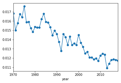
While exploring the data, I noticed that players hit into errors less frequently now than they used to. Let’s see how the probability that a player hits into an error has changed across the years.

1
2
3
4
5
6
7
8
9
10
11
12
%matplotlib inline

YEAR_DF = (DF
           .groupby("year")
           .agg({
               "errors": "sum",
               "bip": "sum"
           })
           .assign(prop_error=lambda x: x["errors"] / x["bip"])
          )

YEAR_DF["prop_error"].plot(style="o-");

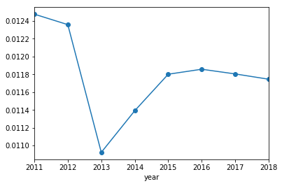
Interestingly, the proportion of errors per BIP has been dropping over time. I am not sure if this is a conscious effort by MLB score keepers, a change in how hitters hit, or improved fielding (but I suspect it’s the score keepers). It looks like this drop in errors per BIP leveled off around 2015. Zooming in.

1
YEAR_DF[YEAR_DF.index > 2010]["prop_error"].plot(style="o-");

I explore this statistically in a jupyter notebook on my github.

Because I don’t want year to confound the analysis, I remove all data before 2015.

1
DF = DF[DF["year"] >= 2015]
1
len(DF)
3591

This leaves me with 3500 year, player combinations.

Next I combine players’ data across years.

1
GROUPED_DF = DF.groupby(["playerid", "player_name"]).agg({"errors": "sum", "bip": "sum"}).reset_index()
1
GROUPED_DF.describe()
errors bip
count 1552.000000 1552.000000
mean 3.835052 324.950387
std 6.073256 494.688755
min 0.000000 1.000000
25% 0.000000 7.000000
50% 1.000000 69.000000
75% 5.000000 437.000000
max 37.000000 2102.000000

I want an idea for how likely players are to hit into errors.

1
2
3
TOTALS = GROUPED_DF.agg({"errors": "sum", "bip": "sum"})
ERROR_RATE = TOTALS["errors"] / TOTALS["bip"]
ERROR_RATE
0.011801960251664112

Again, errors are very rare, so I want know how many “trials” (BIP) I need for a reasonable estimate of how likely each player is to hit into an error.

I’d like the majority of players to have at least 5 errors. I can estimate how many BIP that would require.

1
5. /ERROR_RATE
423.65843413978496

Looks like I should require at least 425 BIP for each player. I round this to 500.

1
GROUPED_DF = GROUPED_DF[GROUPED_DF["bip"] > 500]
1
GROUPED_DF = GROUPED_DF.reset_index(drop=True)
1
GROUPED_DF.head()
playerid player_name errors bip
0 abrej003 Jose Abreu 20 1864
1 adamm002 Matt Adams 6 834
2 adrie001 Ehire Adrianza 2 533
3 aguij001 Jesus Aguilar 2 551
4 ahmen001 Nick Ahmed 12 1101
1
GROUPED_DF.describe()
errors bip
count 354.000000 354.000000
mean 12.991525 1129.059322
std 6.447648 428.485467
min 1.000000 503.000000
25% 8.000000 747.250000
50% 12.000000 1112.000000
75% 17.000000 1475.750000
max 37.000000 2102.000000

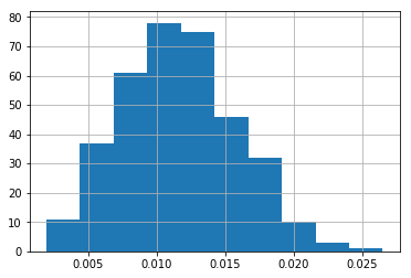
I’ve identified 354 players who have enough BIP for me to estimate how frequently they hit into errors.

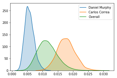
Below, I plot how the likelihood of hitting into errors is distributed.

1
2
3
4
%matplotlib inline

GROUPED_DF["prop_error"] = GROUPED_DF["errors"] / GROUPED_DF["bip"]
GROUPED_DF["prop_error"].hist();

The question is whether someone who has hit into errors in 2% of their BIP is more likely to hit into an error than someone who has hit into errors in 0.5% of their BIP (or is this all just random variation).

To try and estimate this, I treat each BIP as a Bernoulli trial. Hitting into an error is a “success”. I use a Binomial distribution to model the number of “successes”. I would like to know if different players are more or less likely to hit into errors. To do this, I model each player as having their own Binomial distribution and ask whether p (the probability of success) differs across players.

To answer this question, I could use a chi square contingency test but this would only tell me whether players differ at all and not which players differ.

The traditional way to identify which players differ is to do pairwise comparisons, but this would result in TONS of comparisons making false positives all but certain.

Another option is to harness Bayesian statistics and build a Hierarchical Beta-Binomial model. The intuition is that each player’s probability of hitting into an error is drawn from a Beta distribution. I want to know whether these Beta distributions are different. I then assume I can best estimate a player’s Beta distribution by using that particular player’s data AND data from all players together.

The model is built so that as I accrue data about a particular player, I will trust that data more and more, relying less and less on data from all players. This is called partial pooling. Here’s a useful explanation.

I largely based my analysis on this tutorial. Reference the tutorial for an explanation of how I choose my priors. I ended up using a greater lambda value (because the model sampled better) in the Exponential prior, and while this did lead to more extreme estimates of error likelihood, it didn’t change the basic story.

1
2
3
4
5
6
7
8
9
10
11
12
13
14
15
16
17
18
import pymc3 as pm
import numpy as np
import theano.tensor as tt

with pm.Model() as model:

    phi = pm.Uniform('phi', lower=0.0, upper=1.0)

    kappa_log = pm.Exponential('kappa_log', lam=25.)
    kappa = pm.Deterministic('kappa', tt.exp(kappa_log))

    rates = pm.Beta('rates', alpha=phi*kappa, beta=(1.0-phi)*kappa, shape=len(GROUPED_DF))

    trials = np.array(GROUPED_DF["bip"])
    successes = np.array(GROUPED_DF["errors"])

    obs = pm.Binomial('observed_values', trials, rates, observed=successes)
    trace = pm.sample(2000, tune=1000, chains=2, cores=2, nuts_kwargs={'target_accept': .95})
Auto-assigning NUTS sampler...
Initializing NUTS using jitter+adapt_diag...
Multiprocess sampling (2 chains in 2 jobs)
NUTS: [rates, kappa_log, phi]
Sampling 2 chains: 100%|██████████| 6000/6000 [01:47<00:00, 28.06draws/s] 

Check whether the model converged.

1
max(np.max(score) for score in pm.gelman_rubin(trace).values())
1.0022635936332533
1
2
3
bfmi = pm.bfmi(trace)
max_gr = max(np.max(gr_stats) for gr_stats in pm.gelman_rubin(trace).values())
(pm.energyplot(trace, figsize=(6, 4)).set_title("BFMI = {}\nGelman-Rubin = {}".format(bfmi, max_gr)));

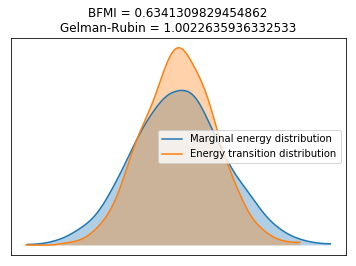
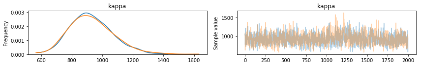
The most challenging parameter to fit is kappa which modulates for the variance in the likelihood to hit into an error. I take a look at it to make sure things look as expected.

1
pm.summary(trace, varnames=["kappa"])
mean sd mc_error hpd_2.5 hpd_97.5 n_eff Rhat
kappa 927.587178 141.027597 4.373954 657.066554 1201.922608 980.288914 1.000013
1
pm.traceplot(trace, varnames=['kappa']);

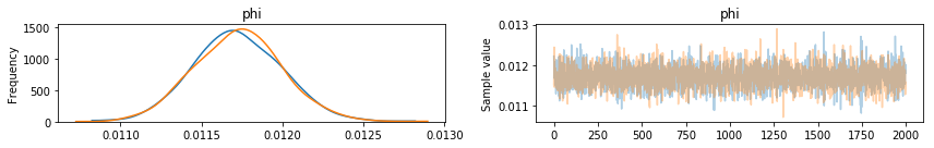
I can also look at phi, the estimated global likelihood to hit into an error.

1
pm.traceplot(trace, varnames=['phi']);

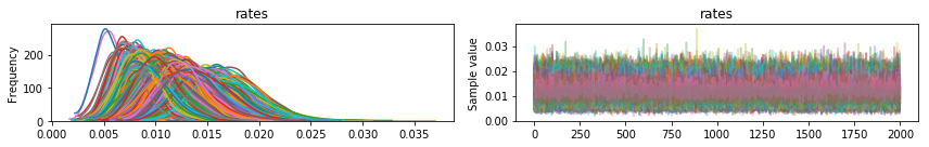
Finally, I can look at how all players vary in their likelihood to hit into an error.

1
pm.traceplot(trace, varnames=['rates']);

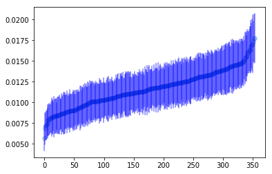
Obviously, the above plot is a lot to look at it, so let’s order players by how likely the model believes they are to hit in an error.

1
2
3
4
5
6
7
8
9
10
11
12
13
14
15
16
from matplotlib import pyplot as plt

rate_means = trace['rates', 1000:].mean(axis=0)
rate_se = trace['rates', 1000:].std(axis=0)

mean_se = [(x, y, i) for i, x, y in zip(GROUPED_DF.index, rate_means, rate_se)]
sorted_means_se = sorted(mean_se, key=lambda x: x[0])
sorted_means = [x[0] for x in sorted_means_se]
sorted_se = [x[1] for x in sorted_means_se]

x = np.arange(len(sorted_means))

plt.plot(x, sorted_means, 'o', alpha=0.25);

for x_val, m, se in zip(x, sorted_means, sorted_se):
    plt.plot([x_val, x_val], [m-se, m+se], 'b-', alpha=0.5)

Now, the ten players who are most likely to hit into an error.

1
2
3
estimated_mean = pm.summary(trace, varnames=["rates"]).iloc[[x[2] for x in sorted_means_se[-10:]]]["mean"]

GROUPED_DF.loc[[x[2] for x in sorted_means_se[-10:]], :].assign(estimated_mean=estimated_mean.values).iloc[::-1]
playerid player_name errors bip prop_error estimated_mean
71 corrc001 Carlos Correa 30 1368 0.021930 0.017838
227 myerw001 Wil Myers 27 1214 0.022241 0.017724
15 andre001 Elvis Andrus 37 1825 0.020274 0.017420
258 plawk001 Kevin Plawecki 14 528 0.026515 0.017200
285 rojam002 Miguel Rojas 21 952 0.022059 0.017001
118 garca003 Avisail Garcia 28 1371 0.020423 0.016920
244 pench001 Hunter Pence 22 1026 0.021442 0.016875
20 baezj001 Javier Baez 23 1129 0.020372 0.016443
335 turnt001 Trea Turner 23 1140 0.020175 0.016372
50 cainl001 Lorenzo Cain 32 1695 0.018879 0.016332

And the 10 players who are least likely to hit in an error.

1
2
3
estimated_mean = pm.summary(trace, varnames=["rates"]).iloc[[x[2] for x in sorted_means_se[:10]]]["mean"]

GROUPED_DF.loc[[x[2] for x in sorted_means_se[:10]], :].assign(estimated_mean=estimated_mean.values)
playerid player_name errors bip prop_error estimated_mean
226 murpd006 Daniel Murphy 4 1680 0.002381 0.005670
223 morrl001 Logan Morrison 4 1241 0.003223 0.006832
343 vottj001 Joey Votto 8 1724 0.004640 0.007112
239 panij002 Joe Panik 7 1542 0.004540 0.007245
51 calhk001 Kole Calhoun 9 1735 0.005187 0.007413
55 carpm002 Matt Carpenter 8 1566 0.005109 0.007534
142 hamib001 Billy Hamilton 8 1476 0.005420 0.007822
289 rosae001 Eddie Rosario 8 1470 0.005442 0.007855
275 renda001 Anthony Rendon 9 1564 0.005754 0.007966
8 alony001 Yonder Alonso 8 1440 0.005556 0.008011

It looks to me like players who hit more ground balls are more likely to hit into an error than players who predominately hits fly balls and line-drives. This makes sense since infielders make more errors than outfielders.

Using the posterior distribution of estimated likelihoods to hit into an error, I can assign a probability to whether Carlos Correa is more likely to hit into an error than Daniel Murphy.

1
np.mean(trace['rates', 1000:][:, 71] <= trace['rates', 1000:][:, 226])
0.0

The model believes Correa is much more likely to hit into an error than Murphy!

I can also plot these players’ posterior distributions.

1
2
3
4
5
import seaborn as sns

sns.kdeplot(trace['rates', 1000:][:, 226], shade=True, label="Daniel Murphy");
sns.kdeplot(trace['rates', 1000:][:, 71], shade=True, label="Carlos Correa");
sns.kdeplot(trace['rates', 1000:].flatten(), shade=True, label="Overall");

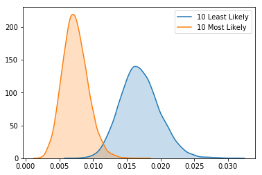
Finally, I can look exclusively at how the posterior distributions of the ten most likely and 10 least likely players to hit into an error compare.

1
2
sns.kdeplot(trace['rates', 1000:][:, [x[2] for x in sorted_means_se[-10:]]].flatten(), shade=True, label="10 Least Likely");
sns.kdeplot(trace['rates', 1000:][:, [x[2] for x in sorted_means_se[:10]]].flatten(), shade=True, label="10 Most Likely");

All in all, this analysis makes it obvious that some players are more likely to hit into errors than other players. This is probably driven by how often players hit ground balls.

Data Science Lessons Learned the Hard Way: Coding

You could summarize this post as “you will never regret good code practices” or “no project is too small for good code practices”.

You might think these recommendations are not worth the time when a project seems small, but projects often grow over time. If you use good practices from the start, you will reduce the technical debt your project accrues over time.

Here’s my list of coding Data Science lessons learned the hard way.

  1. You will never regret using git.

    You might think, “this project/query is just 15 minutes of code and I will never think about it again”. While this might be true, it often is not. If your project/query is useful, people will ask for it again with slight tweaks. With each ask, the project grows a little. By using git, you persist the project at all change points, acknowledge that the project will change over time, and prepare for multiple contributors.
    Even if you never use these features, I’ve found that simply using git encourages other good practices. Also, remember git can rescue you when things go wrong!

  2. You will never regret good documentation.

    Again, you might think, “this project is so tiny and simple, how could I ever forget how it works??”. You will forget. Or another contributor will appreciate documentation.
    The numpy documentation framework is great when working in python. Its integration with sphinx can save you a lot of time when creating non-code documentation.
    I recently started documenting not only what the code is doing, but the business rule dictating what the code should do. Having both lets contributors know not only know the how of the code but also the why.

  3. You will never regret building unit-tests.

    Again, this might feel like over-kill in small projects, but even small projects have assumptions that should be tested. This is especially true when you add new features after stepping away from a project. By including unit-tests, you assure yourself that existing features did not break, making those pushes to production less scary.

  4. Take the time to build infrastructure for gathering/generating sample/fake data.

    I’ve found myself hesitant to build unit-tests because it’s hard to acquire/generate useful sample/fake data. Do not let this be a blocker to good code practices! Take the time to build infrastructure that makes good code practices easy. This could mean taking the time to write code for building fake data. This could mean taking the time to acquire useful sample data. Maybe it’s both! Take the time to do it. You will not regret making it easy to write tests.

  5. You will always find a Makefile useful.

    Once you’ve built infrastructure for acquiring fake or sample data, you will need a way to bring this data into your current project. I’ve found Makefiles useful for this sort of thing. You can define a command that will download some sample data from s3 (or wherever) and save it to your repo (but don’t track these files on git!).
    This way all contributors will have common testing data, stored outside of git, and can acquire this data with a single, easy to remember, command.
    MakeFiles are also great for installing or saving a project’s dependencies.

  6. Know your project’s dependencies.

    Code ecosystems change over time. When you revisit a project after a break, the last thing you want is to guess what code dependencies have broken. It doesn’t matter whether you save your project’s dependencies as a anaconda environment, a requirements file, virtualenv, a docker image, whatever. Just make sure to save it. Any future contributors (including yourself!!) will thank you.

Most these individual points seem obvious. The overarching point is no project is too small for good code practices. Sure you might think, oh this is just a single query, but you will run that query again, or another member of your team will! While you shouldn’t build a repo for each query, building a repo for different sets of queries is not a bad idea.

Are Some Mlb Players More Likely to Hit Into Errors Than Others: Data Munging

I recently found myself wondering if some baseball players are more likely to hit into errors than others. In theory, the answer should be “no” since fielders produce errors regardless of who is hitting. Nonetheless, it’s also possible that some hitters “force” errors by hitting the ball harder or running to first base faster.

In order to evaluate this possibility, I found play-by-play data on retrosheet.org. This data contains row by row data describing each event (e.g., a hit, stolen base etc) in a baseball game. I’ve posted this analysis on github and will walk through it here.

The user is expected to input what year’s data they want. I write the code’s output for the year 2018 as comments. The code starts by downloading and unzipping the data.

1
2
3
4
5
6
7
8
9
YEAR=$1
FILE_LOC=https://www.retrosheet.org/events/${YEAR}eve.zip

echo "---------DOWNLOAD----------"
wget -nc $FILE_LOC -O ./raw_data/${YEAR}.zip

echo "---------UNPACK----------"
mkdir raw_data/${YEAR}/
unzip -o raw_data/${YEAR}.zip -d raw_data/${YEAR}/

The unzipped data contain play-by-play data in files with the EVN or EVA extensions. Each team’s home stadium has its own file. I combine all the play-by play eveSSplants (.EVN and .EVA files) into a single file. I then remove all non batting events (e.g., balk, stolen base etc).

I also combine all the roster files (.ROS) into a single file.

1
2
3
4
5
6
7
8
9
10
11
12
13
14
15
16
17
# export playbyplay to single file
mkdir processed_data/${YEAR}/
find raw_data/${YEAR}/ -regex '.*EV[A|N]' | \
	xargs grep play > \
	./processed_data/${YEAR}/playbyplay.out

# get all plate appearances from data (and hitter). remove all non plate appearance rows
cat ./processed_data/${YEAR}/playbyplay.out | \
	awk -F',' '{print $4","$7}' | \
	grep -Ev ',[A-Z]{3}[0-9]{2}' | \
	grep -Ev ',(NP|BK|CS|DI|OA|PB|WP|PO|POCS|SB|FLE)' > \
	./processed_data/${YEAR}/batters.out

# one giant roster file
find raw_data/${YEAR}/ -name '*ROS' | \
	xargs awk -F',' '{print $1" "$2" "$3}' > \
	./processed_data/${YEAR}/players.out

In this next few code blocks I print some data just to see what I am working with. For instance, I print out players with the most plate appearances. I was able to confirm these numbers with baseball-reference. This operation requires me to groupby player and count the rows. I join this file with the roster file to get player’s full names.

1
2
3
4
5
6
7
8
9
10
11
12
13
14
15
16
17
18
19
20
21
22
23
echo "---------PLAYERS WITH MOST PLATE APPEARANCES----------"
cat ./processed_data/${YEAR}/batters.out | \
	awk -F, '{a[$1]++;}END{for (i in a)print i, a[i];}' | \
	sort -k2 -nr | \
	head > \
	./processed_data/${YEAR}/most_pa.out
join <(sort -k 1 ./processed_data/${YEAR}/players.out) <(sort -k 1 ./processed_data/${YEAR}/most_pa.out) | \
	uniq | \
	sort -k 4 -nr | \
	head | \
	awk '{print $3", "$2", "$4}'

#---------PLAYERS WITH MOST PLATE APPEARANCES----------
#Francisco, Lindor, 745
#Trea, Turner, 740
#Manny, Machado, 709
#Cesar, Hernandez, 708
#Whit, Merrifield, 707
#Freddie, Freeman, 707
#Giancarlo, Stanton, 706
#Nick, Markakis, 705
#Alex, Bregman, 705
#Marcus, Semien, 703

Here’s the players with the most hits. Notice that I filter out all non-hits in the grep, then group by player.

1
2
3
4
5
6
7
8
9
10
11
12
13
14
15
16
17
18
echo "---------PLAYERS WITH MOST HITS----------"
cat ./processed_data/${YEAR}/batters.out | \
	grep -E ',(S|D|T|HR)' | \
	awk -F, '{a[$1]++;}END{for (i in a)print i, a[i];}' | \
	sort -k2 -nr | \
	head

#---------PLAYERS WITH MOST HITS----------
#merrw001 192
#freef001 191
#martj006 188
#machm001 188
#yelic001 187
#markn001 185
#castn001 185
#lindf001 183
#peraj003 182
#blacc001 182

Here’s the players with the most at-bats.

1
2
3
4
5
6
7
8
9
10
11
12
13
14
15
16
17
18
19
echo "---------PLAYERS WITH MOST AT BATS----------"
cat ./processed_data/${YEAR}/batters.out | \
	grep -Ev 'SF|SH' | \
	grep -E ',(S|D|T|HR|K|[0-9]|E|DGR|FC)' | \
	awk -F, '{a[$1]++;}END{for (i in a)print i, a[i];}' > \
	./processed_data/${YEAR}/abs.out
cat ./processed_data/${YEAR}/abs.out | sort -k2 -nr | head

#---------PLAYERS WITH MOST AT BATS----------
#turnt001 664
#lindf001 661
#albio001 639
#semim001 632
#peraj003 632
#merrw001 632
#machm001 632
#blacc001 626
#markn001 623
#castn001 620

And, finally, here’s the players who hit into the most errors.

1
2
3
4
5
6
7
8
9
10
11
12
13
14
15
16
17
18
19
echo "---------PLAYERS WHO HIT INTO THE MOST ERRORS----------"
cat ./processed_data/${YEAR}/batters.out | \
    	grep -Ev 'SF|SH' | \
	grep ',E[0-9]' | \
	awk -F, '{a[$1]++;}END{for (i in a)print i, a[i];}' > \
	./processed_data/${YEAR}/errors.out
cat ./processed_data/${YEAR}/errors.out | sort -k2 -nr | head

#---------PLAYERS WHO HIT INTO THE MOST ERRORS----------
#gurry001 13
#casts001 13
#baezj001 12
#goldp001 11
#desmi001 11
#castn001 10
#bogax001 10
#andum001 10
#turnt001 9
#rojam002 9

Because players with more at-bats hit into more errors, I need to take the number of at-bats into account. I also filter out all players with less than 250 at bats. I figure we only want players with lots of opportunities to create errors.

1
2
3
4
5
6
7
8
9
10
11
12
13
14
15
16
17
18
echo "---------PLAYERS WITH MOST ERRORS PER AT BAT----------"
join -e"0" -a1 -a2 <(sort -k 1 ./processed_data/${YEAR}/abs.out) -o 0 1.2 2.2 <(sort -k 1 ./processed_data/${YEAR}/errors.out) | \
	uniq | \
	awk -v OFS=', ' '$2 > 250 {print $1, $3, $2, $3/$2}' >  \
	./processed_data/${YEAR}/errors_abs.out
cat ./processed_data/${YEAR}/errors_abs.out | sort -k 4 -nr | head

#---------PLAYERS WITH MOST ERRORS PER AT BAT----------
#pereh001, 8, 316, 0.0253165
#gurry001, 13, 537, 0.0242086
#andre001, 9, 395, 0.0227848
#casts001, 13, 593, 0.0219224
#desmi001, 11, 555, 0.0198198
#baezj001, 12, 606, 0.019802
#garca003, 7, 356, 0.0196629
#bogax001, 10, 512, 0.0195312
#goldp001, 11, 593, 0.0185497
#iglej001, 8, 432, 0.0185185

At-bats is great but even better is to remove strike-outs and just look at occurences when a player hit the ball into play. I remove all players with less than 450 balls hit into play which limits us to just 37 players but the players have enough reps to make the estimates more reliable.

1
2
3
4
5
6
7
8
9
10
11
12
13
14
15
16
17
18
19
20
21
22
23
echo "---------PLAYERS WITH MOST ERRORS PER BALL IN PLAY----------"
cat ./processed_data/${YEAR}/batters.out | \
	grep -Ev 'SF|SH' | \
	grep -E ',(S|D|T|HR|[0-9]|E|DGR|FC)' | \
	awk -F, '{a[$1]++;}END{for (i in a)print i, a[i];}' > \
	./processed_data/${YEAR}/bip.out
join -e"0" -a1 -a2 <(sort -k 1 ./processed_data/${YEAR}/bip.out) -o 0 1.2 2.2 <(sort -k 1 ./processed_data/${YEAR}/errors.out) | \
	uniq | \
	awk -v OFS=', ' '$2 > 450 {print $1, $3, $2, $3/$2}' > \
	./processed_data/${YEAR}/errors_bip.out
cat ./processed_data/${YEAR}/errors_bip.out | sort -k 4 -nr | head

#---------PLAYERS WITH MOST ERRORS PER BALL IN PLAY----------
#casts001, 13, 469, 0.0277186
#gurry001, 13, 474, 0.0274262
#castn001, 10, 469, 0.021322
#andum001, 10, 476, 0.0210084
#andeb006, 9, 461, 0.0195228
#turnt001, 9, 532, 0.0169173
#simma001, 8, 510, 0.0156863
#lemad001, 7, 451, 0.0155211
#sancc001, 7, 462, 0.0151515
#freef001, 7, 486, 0.0144033

Now we have some data. In future posts I will explore how we can use statistics to evaluate whether some players are more likely to hit into errors than others.

Check out the companion post that statistically explores this question.

Complex Aggregations in PySpark

I’ve touched on this in past posts, but wanted to write a post specifically describing the power of what I call complex aggregations in PySpark.

The idea is that you have have a data request which initially seems to require multiple different queries, but using ‘complex aggregations’ you can create the requested data using a single query (and a single shuffle).

Let’s say you have a dataset like the following. You have one column (id) which is a unique key for each user, another column (group) which expresses the group that each user belongs to, and finally (value) which expresses the value of each customer. I apologize for the contrived example.

1
2
3
4
5
6
7
8
9
10
11
12
13
from pyspark.sql import functions as F
from pyspark.sql import types as T
from pyspark.sql import SparkSession
from pyspark import SparkContext

sc = SparkContext("local", "Example")
spark = SparkSession(sc)

a = sc.parallelize([[1, 'a', 5.1],
                    [2, 'b', 2.6],
                    [3, 'b', 3.4],
                    [4, 'c', 1.7]]).toDF(['id', 'group', 'value'])
a.show()
id group value
1 'a' 5.1
2 'b' 2.6
3 'b' 3.4
4 'c' 1.7

Let’s say someone wants the average value of group a, b, and c, AND the average value of users in group a OR b, the average value of users in group b OR c AND the value of users in group a OR c. Adds a wrinkle, right? The ‘or’ clauses prevent us from using a simple groupby, and we don’t want to have to write 4 different queries.

Using complex aggregations, we can access all these different conditions in a single query.

1
2
3
4
5
6
7
8
9
10
11
12
13
14
15
16
17
18
19
20
21
final_data = (a
              .agg(
                F.avg(F.when(F.col('group') == 'a', F.col('value')).otherwise(None)).alias('group_a_avg'),
                F.avg(F.when(F.col('group') == 'b', F.col('value')).otherwise(None)).alias('group_b_avg'),
                F.avg(F.when(F.col('group') == 'c', F.col('value')).otherwise(None)).alias('group_c_avg'),
                F.avg((F.when(F.col('group') == 'a', F.col('value'))
                        .when(F.col('group') == 'b', F.col('value'))
                        .otherwise(None)
                      )).alias('group_ab_avg'),
                F.avg((F.when(F.col('group') == 'b', F.col('value'))
                        .when(F.col('group') == 'c', F.col('value'))
                        .otherwise(None)
                      )).alias('group_bc_avg'),
                F.avg((F.when(F.col('group') == 'a', F.col('value'))
                        .when(F.col('group') == 'c', F.col('value'))
                        .otherwise(None)
                      )).alias('group_ac_avg'),
                )
              )

final_data.show()
group_a_avg group_b_avg group_c_avg group_ab_avg group_ac_avg group_bc_avg
5.1 3.0 1.7 3.7 3.4 2.6

They key here is using when to filter different data in and out of different aggregations.

This approach can be quite concise when used with python list comprehensions. I’ll rewrite the query above, but using a list comprehension.

1
2
3
4
5
6
7
8
9
10
11
from itertools import combinations

groups  = ['a', 'b', 'c']
combos = [x for x in combinations(groups,  2)]
print(combos)
#[('a', 'b'), ('a', 'c'), ('b', 'c')]

single_group = [F.avg(F.when(F.col('group') == x, F.col('value')).otherwise(None)).alias('group_%s_avg' % x) for x in groups]
double_group = [F.avg(F.when(F.col('group') == x, F.col('value')).when(F.col('group')==y, F.col('value')).otherwise(None)).alias('group_%s%s_avg' % (x, y)) for x, y in combos]
final_data = a.agg(*single_group + double_group)
final_data.show()
group_a_avg group_b_avg group_c_avg group_ab_avg group_ac_avg group_bc_avg
5.1 3.0 1.7 3.7 3.4 2.6

Voila! Hope you find this little trick helpful! Let me know if you have any questions or comments.

Introducing Predeval

Predeval is software designed to help you identify changes in a model’s output.

For instance, you might be tasked with building a model to predict churn. When you deploy this model in production, you have to wait to learn which users churned in order to know how your model performed. While Predeval will not free you from this wait, it can provide initial signals as to whether the model is producing reasonable (i.e., expected) predictions. Unexpected predictions might reflect a poor performing model. They also might reflect a change in your input data. Either way, something has changed and you will want to investigate further.

Using predeval, you can detect changes in model output ASAP. You can then use python’s libraries to build a surrounding alerting system that will signal a need to investigate. This system should give you additional confidence that your model is performing reasonably. Here’s a post where I configure an alerting system using python, mailutils, and postfix (although the alerting system is not built around predeval).

Predeval operates by forming expectations about what your model’s outputs will look like. For example, you might give predeval the model’s output from a validation dataset. Predeval will then compare new outputs to the outputs produced by the validation dataset, and will report whether it detects a difference.

Predeval works with models producing both categorical and continuous outputs.

Here’s an example of predeval with a model producing categorical outputs. Predeval will (by default) check whether all expected output categories are present, and whether the output categories occur at their expected frequencies (using a Chi-square test of independence of variables in a contingency table).

Here’s an example of predeval with a model producing continuous outputs. Predeval will (by default) check whether the new output have a minimum lower than expected, a maximum greater than expected, a different mean, a different standard deviation, and whether the new output are distributed as expected (using a Kolmogorov-Smirnov test)

I’ve tried to come up with reasonable defaults for determining whether data are different, but you can also set these thresholds yourself. You can also choose what comparison tests to run (e.g., checking the minimum, maximum etc.).

You will likely need to save your predeval objects so that you can apply them to future data. Here’s an example of saving the objects.

Documentation about how to install predeval can be found here.

If you have comments about improvements or would like to contribute, please reach out!