This is the second post in a series of posts about moving from a PhD in Psychology/Cognitive Psychology/Cognitive Neuroscience to data science. The first post answers many of the best and most common questions I’ve heard about my transition. This post focuses on the technical skills that are often necessary for landing a data science job.

Each header in this post represents a different technical area. Following the header I describe what I would know before walking into an interview.

SQL

SQL is not often used in academia, but it’s probably the most important skill in data science (how do you think you’ll get your data??). It’s used every day by data scientists at every company, and while it’s 100% necessary to know, it’s stupidly boring to learn. But, once you get the hang of it, it’s a fun language because it requires a lot of creativity. To learn SQL, I would start by doing the mode analytics tutorials, then the sql zoo problems. Installing postgres on your personal computer and fetching data in Python with psycopg2 or sql-alchemy is a good idea. After, completing all this, move onto query optimization (where the creativity comes into play) - check out the explain function and order of execution. Shameless self promotion: I made a SQL presentation on what SQL problems to know for job interviews.

Python/R

Some places use R. Some places use Python. It sucks, but these languages are not interchangeable (an R team will not hire someone who only knows Python). Whatever language you choose, you should know it well because this is a tool you will use every day. I use Python, so what follows is specific to Python.

I learned Python with codeacademy and liked it. If you’re already familiar with Python I would practice “white board” style questions. Feeling comfortable with the beginner questions on a site like leetcode or hackerrank would be a good idea. Writing answers while thinking about code optimization is a plus.

Jeff Knupp’s blog has great tid-bits about developing in python; it’s pure gold.

Another good way to learn is to work on your digital profile. If you haven’t already, I would start a blog (I talk more about this is Post 1).

Statistics/ML

When starting here, the Andrew Ng coursera course is a great intro. While it’s impossible to learn all of it, I love to use elements of statistical learning and it’s sibling book introduction to statistical learning as a reference. I’ve heard good things about Python Machine Learning but haven’t checked it out myself.

As a psychology major, I felt relatively well prepared in this regard. Experience with linear-mixed effects, hypothesis-testing, regression, etc. serves Psychology PhDs well. This doesn’t mean you can forget Stats 101 though. Once, I found myself uncomfortably surprised by a very basic probability question.

Here’s a quick list of Statistics/ML algorithms I often use: GLMs and their regularization methods are a must (L1 and L2 regularization probably come up in 75% of phone screens). Hyper-parameter search. Cross-validation! Tree-based models (e.g., random forests, boosted decision trees). I often use XGBoost and have found its intro post helpful.

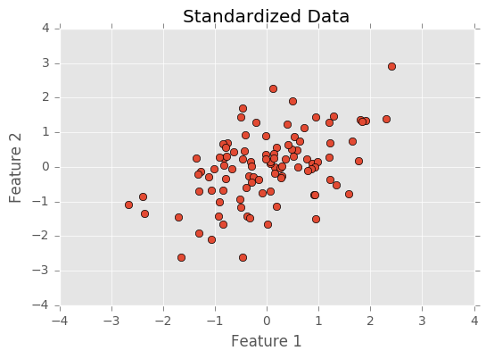
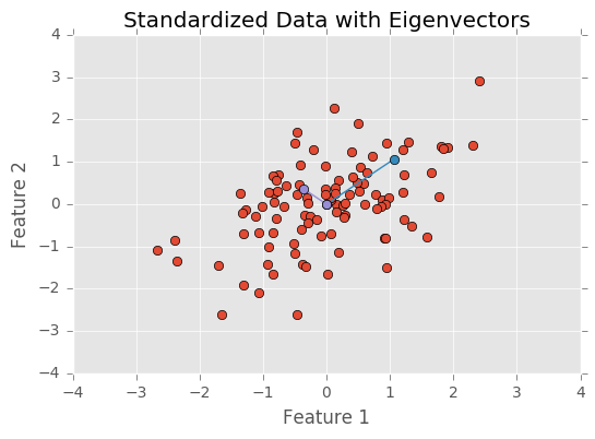
I think you’re better off deeply (pun not intended) learning the basics (e.g., linear and logistic regression) than learning a smattering of newer, fancier methods (e.g., deep learning). This means thinking about linear regression from first principles (what are the assumptions and given these assumptions can you derive the best-fit parameters of a linear regression?). I can’t tell you how many hours I’ve spent studying Andrew Ng’s first supervised learning lecture for this. It’s good to freshen up on linear algebra and there isn’t a better way to do this than the 3Blue1Brown videos; they’re amazing. This might seem too introductory/theoretical, but it’s necessary and often comes up in interviews.

Be prepared to talk about the bias-variance tradeoff. Everything in ML comes back to the bias-variance tradeoff so it’s a great interview question. I know some people like to ask candidates about feature selection. I think this question is basically a rephrasing of the bias-variance tradeoff.

Git/Code Etiquette

Make a github account if you haven’t already. Get used to commits, pushing, and branching. This won’t take long to get the hang of, but, again, it’s something you will use every day.

As much as possible I would watch code etiquette. I know this seems anal, but it matters to some people (myself included), and having pep8 quality code can’t hurt. There’s a number of python modules that will help here. Jeff Knupp also has a great post about linting/automating code etiquette.

Unit-tests are a good thing to practice/be familiar with. Like usual, Jeff Knupp has a great post on the topic.

I want to mention that getting a data science job is a little like getting a grant. Each time you apply, there is a low chance of getting the job/grant (luckily, there are many more jobs than grants). When creating your application/grant, it’s important to find ways to get people excited about your application/grant (e.g., showing off your statistical chops). This is where code etiquette comes into play. The last thing you want is to diminish someone’s excitement about you because you didn’t include a doc string. Is code etiquette going to remove you from contention for a job? Probably not. But it could diminish someone’s excitement.

Final Thoughts

One set of skills that I haven’t touched on is cluster computing (e.g., Hadoop, Spark). Unfortunately, I don’t think there is much you can do here. I’ve heard good things about the book Learning Spark, but books can only get you so far. If you apply for a job that wants Spark, I would install Spark on your local computer and play around, but it’s hard to learn cluster computing when you’re not on a cluster. Spark is more or less fancy SQL (aside from the ML aspects), so learning SQL is a good way to prepare for a Spark mindset. I didn’t include cluster computing above, because many teams seem okay with employees learning this on the job.

Not that there’s a lack of content here, but here’s a good list of must know topics that I used when transitioning from academia to data science.

A number of people have asked about moving from a PhD in Psychology/Cognitive Psychology/Cognitive Neuroscience to data science. This blog post is part of a 2-part series where I record my answers to the best and most common questions I’ve heard. Part 2 can be found here.

Before I get started, I want to thank Rick Wolf for providing comments on an earlier version of this post.

This first post is a series of general questions I’ve received. The second post will focus on technical skills required to get a job in data science.

Each header in this post represents a question. Below the header/question I record my response.

Anyone starting this process should know they are starting a marathon. Not a sprint. Making the leap from academia to data science is more than possible, but it takes time and dedication.

Do you think that being a Psychology PhD is a disadvantage?

I think it can be a disadvantage in the job application process. Most people don’t understand how quantitative Psychology is, so psychology grads have to overcome these stereotypes. This doesn’t mean having a Psychology PhD is a disadvantage when it comes to BEING a data scientist. Having a Psychology PhD can be a huge advantage because Psychology PhDs have experience measuring behavior which is 90% of data science. Every company wants to know what their customers are doing and how to change their customers’ behavior. This is literally what Psychology PhDs do, so Psychology PhDs might have the most pertinent experience of any science PhD.

When it is the right time to apply for a boot camp?

(I did the Insight Data Science bootcamp)
Apply when you’re good enough to get a phone screen but not good enough to get a job. Don’t count on a boot camp to give you all the skills. Instead, think of boot camps as polishing your skills.

Here is the game plan I would use:
Send out 3-4 job applications and see if you get any hits. If not, think about how you can improve your resume (see post #2), and go about those improvements. After a few iterations of this, you will start getting invitations to do phone screens. At this stage, a boot camp will be useful.
The boot camps are of varying quality. Ask around to get an idea for which boot camps are better or worse. Also, look into how each boot camp gets paid. If you pay tuition, the boot camp will care less about whether you get a job. If the boot camp gets paid through recruiting fees or collecting tuition from your paychecks, it is more invested in your job.

Should I start a blog?

Yes, I consider this a must (and so do others). It’s a good opportunity to practice data science, and, more importantly, it’s a good opportunity to show off your skills.

Most people (including myself) host their page on github and generate the html with a static site generator. I use octopress, which works great. Most people seem to use pelican. I would recommend pelican because it’s built in Python. I haven’t used it, but a quick google search led me to this tutorial on building a github site with pelican.

I wish I’d sent more of my posts to friends/colleagues. Peer review is always good for a variety of reasons. I’d be more than happy to review posts for anyone reading this blog.

How should I frame what I’ve done in academia on my CV/resume?

First, no one in industry cares about publications. People might notice if the journal is Science/Nature but most will not. Spend a few hours thinking about how to describe your academic accomplishments as technical skills. For example, as a Postdoc, I was on a Neurophysiology project that required writing code to collect, ingest, and transform electrophysiology data. In academia, none of this code mattered. In industry, it’s the only thing that matters. What I built was a data-pipeline, and this is a product many companies desire.

We all have examples like this, but they’re not obvious because academics don’t know what companies want. Think of your data-pipelines, your interactive experiments, your scripted analytics.

Transforming academic work into skills that companies desire will take a bit of creativity (I am happy to help with this), but remember that your goal here is to express how the technical skills you used in academia will apply to what you will do as a data scientist.

Many people (including myself) love to say they can learn fast. While this is an important skill it’s hard to measure and it calls attention to what you do not know. In general, avoid it.

Did you focus on one specific industry?

I think a better question than what industry is what size of team/company you want to work on. At a big company you will have a more specific job with more specific requirements (and probably more depth of knowledge). At a smaller company, you will be expected to have a broader skill set. This matters in terms of what you want in a job and what skills you have. Having industry specific knowledge is awesome, but most academics have never worked in an industry so by definition they don’t have industry specific knowledge. Unfortunately, we just have to punt on this aspect of the job application.

Anything to be wary of?

No matter what your job is, having a good boss is important. If you get a funny feeling about a potential boss in the interview process, don’t take the job.

Some companies are trying to hire data scientists but don’t want to change their company. By this I mean they want their data scientists to work in excel. Excel is a great tool, but it’s not a tool I would want to use every day. If you feel the same way, then keep an eye out for this.

I recently spent an entire afternoon debugging a solution for automatically launching a weekly emr job.

Hopefully, I can save someone the same pain by writing this blog post.

I decided to use Cron to launch the weekly jobs. Actually launching a weekly job on Cron was not difficult. Check out the Ubuntu Cron manual for a good description on how to use Cron.

What took me forever was realizing that Cron jobs have an extremely limited path. Because of this, specifying the complete path to executed files and their executors is necessary.

Below I describe how I used an ec2 instance (Ubuntu 16.04) to automatically launch this weekly job.

First, here is what my Cron job list looks like (call “crontab -e” in the terminal).

1
2

SHELL=/bin/bash
05 01 * * 2 $HOME/automated_jobs/production_cluster.sh

The important thing to note here is that I am creating the variable SHELL, and $HOME is replaced by the actual path to my home directory.

Next, is the shell script called by Cron.

1
2
3
4

#!/bin/bash
source $HOME/.bash_profile

python $HOME/automated_jobs/launch_production_cluster.py

Again, $HOME is replaced with the actual path to my home directory.

I had to make this shell script and the python script called within it executable (call “chmod +x” in the terminal). The reason that I used this shell script rather than directly launching the python script from Cron is I wanted access to environment variables in my bash_profile. In order to get access to them, I had to source bash_profile.

Finally, below I have the python file that executes the week job that I wanted. I didn’t include the code that actually launches our emr cluster because that wasn’t the hard part here, but just contact me if you would like to see it.

1
2
3
4
5
6
7
8
9
10
11
12
13
14
15
16
17
18
19
20
21
22
23
24

#!$HOME/anaconda2/bin/python
import os
import sys
import datetime as dt
from subprocess import check_output

# setup logging
old_stdout = sys.stdout
log_file = open("production_cluster_%s.log" % dt.datetime.today().strftime('%Y_%m_%d'), "w")
sys.stdout = log_file

print 'created log file'

# organize local files and s3 files

print 'organized files'

# call emr cluster

print 'launched production job'

# close log file
sys.stdout = old_stdout
log_file.close()

While the code is not included here, I use aws cli to launch my emr cluster, and I had to specify the path to aws (call “which aws” in the terminal) when making this call.

You might have noticed the logging I am doing in this script. I found logging both within this python script and piping the output of this script to additional logs helpful when debugging.

The Ubuntu Cron manual I linked above, makes it perfectly clear that my Cron path issues are common, but I wanted to post my solution in case other people needed a little guidance.

I recently found myself in a argument with my wife regarding whether TV was better now than previously. I believed that TV was better now than 20 years ago. My wife contended that there was simply more TV content being produced, and that this led to more good shows, but shows are not inherently any better.

This struck me as a great opportunity to do some quick data science. For this post, I scraped the names (from wikipedia) and ratings (from TMDb) of all American TV shows. I did the same for major American movies, so that I could have a comparison group (maybe all content is better or worse). The ratings are given by TMDb’s users and are scores between 1 and 10 (where 10 is a great show/movie and 1 is a lousy show/movie).

All the code for this post can be found on my github.

I decided to operationalize my “golden age of TV” hypothesis as the average TV show is better now than previously. This would be expressed as a positive slope (beta coefficient) when building a linear regression that outputs the rating of a show given the date on which the show first aired. My wife predicted a slope near zero or negative (shows are no better or worse than previously).

Below, I plot the ratings of TV shows and movies across time. Each show is a dot in the scatter plot. Show rating (average rating given my TMBb) is on the y-axis. The date of the show’s first airing is on the x-axis. When I encountered shows with the same name, I just tacked a number onto the end. For instance, show “x” would become show “x_1.” The size of each point in the scatter plot is the show’s “popularity”, which is a bit of a black box, but it’s given by TMBb’s API. TMDb does not give a full description of how they calculate popularity, but they do say its a function of how many times an item is viewed on TMDb, how many times an item is rated, and how many times the item has been added to watch or favorite list. I decided to depict it here just to give the figures a little more detail. The larger the dot, the more popular the show.

Here’s a plot of all TV shows across time.

To test the “golden age of TV” hypothesis, I coded up a linear regression in javascript (below). I put the regression’s output as a comment at the end of the code. Before stating whether the hypothesis was rejected or not, I should note that that I removed shows with less than 10 votes because these shows had erratic ratings.

As you can see, there is no evidence that TV is better now that previously. In fact, if anything, this dataset says that TV is worse (but more on this later).

1
2
3
4
5
6
7
8
9
10
11
12
13
14
15
16
17
18
19
20
21
22
23
24
25
26
27
28
29
30
31
32
33
34
35

function linearRegression(y,x){

    var lr = {};
    var n = y.length;
    var sum_x = 0;
    var sum_y = 0;
    var sum_xy = 0;
    var sum_xx = 0;
    var sum_yy = 0;

    for (var i = 0; i < y.length; i++) {

        sum_x += x[i];
        sum_y += y[i];
        sum_xy += (x[i]*y[i]);
        sum_xx += (x[i]*x[i]);
        sum_yy += (y[i]*y[i]);
    }

    lr['slope'] = (n * sum_xy - sum_x * sum_y) / (n*sum_xx - sum_x * sum_x);
    lr['intercept'] = (sum_y - lr.slope * sum_x)/n;
    lr['r2'] = Math.pow((n*sum_xy - sum_x*sum_y)/Math.sqrt((n*sum_xx-sum_x*sum_x)*(n*sum_yy-sum_y*sum_y)),2);

    return lr;

};

var yval = data
    .filter(function(d) { return d.vote_count > 10 })
    .map(function (d) { return parseFloat(d.vote_average); });
var xval = data
    .filter(function(d) { return d.vote_count > 10 })
    .map(function (d) { return d.first_air_date.getTime() / 1000; });
var lr = linearRegression(yval,xval);
// Object { slope: -3.754543948800799e-10, intercept: 7.0808230581192815, r2: 0.038528573017115 }

I wanted to include movies as a comparison to TV. Here’s a plot of all movies across time.

It’s important to note that I removed all movies with less than 1000 votes. This is completely 100% unfair, BUT I am very proud of my figures here and things get a little laggy when including too many movies in the plot. Nonetheless, movies seem to be getting worse over time! More dramatically than TV shows!

1
2
3
4
5
6
7
8

var yval = data
    .filter(function(d) { return d.vote_count > 1000 })
    .map(function (d) { return parseFloat(d.vote_average); });
var xval = data
    .filter(function(d) { return d.vote_count > 1000 })
    .map(function (d) { return d.first_air_date.getTime() / 1000; });
var lr = linearRegression(yval,xval);
// Object { slope: -8.11645196776367e-10, intercept: 7.659366705415847, r2: 0.16185069580043676 }

Okay, so this was a fun little analysis, but I have to come out and say that I wasn’t too happy with my dataset and the conclusions we can draw from this analysis are only as good as the dataset.

The first limitation is that recent content is much more likely to receive a rating than older content, which could systematically bias the ratings of older content (e.g., only good shows from before 2000 receive ratings). It’s easy to imagine how this would lead us to believing that all older content is better than it actually was.

Also, TMDb seems to have IMDB type tastes by which I mean its dominated by young males. For instance, while I don’t like the show “Keeping up the Kardashians,” it’s definitely not the worst show ever. Also, “Girls” is an amazing show which gets no respect here. The quality of a show is in the eye of the beholder, which in this case seems to be boys.

I would have used Rotten Tomatoes’ API, but they don’t provide access to TV ratings.

Even with all these caveats in mind, it’s hard to defend my “golden age of TV” hypothesis. Instead, it seems like there is just more content being produced, which leads to more good shows (yay!), but the average show is no better or worse than previously.

NOTE: Since writing this post, PBS Newshour changed their site. They know use the url, https://www.pbs.org/newshour/video. The mechanics here will work but the url has changed and some of the queries need to be changed too. Check the repo for a working version of the code.

I’ve been using Kodi/XBMC since 2010. It provides a flexible and (relatively) intuitive interface for interacting with content through your TV (much like an apple TV). One of the best parts of Kodi is the addons - these are apps that you can build or download. For instance, I use the NBA League Pass addon for watching Wolves games. I’ve been looking for a reason to build my own Kodi addon for years.

Enter PBS NewsHour. If you’re not watching PBS NewsHour, I’m not sure what you’re doing with your life because it’s the shit. It rocks. PBS NewsHour disseminates all their content on youtube and their website. For the past couple years, I’ve been watching their broadcasts every morning through the Youtube addon. This works fine, but it’s clunky. I decided to stream line watching the NewsHour by building a Kodi addon for it.

I used this tutorial to build a Kodi addon that accesses the PBS NewsHour content through the youtube addon. This addon can be found on my github. The addon works pretty well, but it includes links to all NewsHour’s content, and I only want the full episodes. I am guessing I could have modified this addon to get what I wanted, but I really wanted to build my own addon from scratch.

The addon I built is available on my github. To build my addon, I used this tutorial, and some code from this github repository. Below I describe how the addon works. I only describe the file default.py because this file does the majority of the work, and I found the linked tutorials did a good job explaining the other files.

I start by importing libraries that I will use. Most these libraries are used for scraping content off the web. I then create some basic variables to describe the addon’s name (addonID), its name in kodi (base_url), the number used to refer to it (addon_handle - I am not sure how this number is used), and current arguments sent to my addon (args).

1
2
3
4
5
6
7
8
9
10
11
12
13
14
15
16

import zlib
import json
import sys
import urlparse
import xbmc
import xbmcgui
import xbmcplugin

import urllib2
import re

addonID = 'plugin.video.pbsnewshour'

base_url = sys.argv[0]
addon_handle = int(sys.argv[1])
args = urlparse.parse_qs(sys.argv[2][1:])

The next function, getRequest, gathers html from a website (specified by the variable url). The dictionary httpHeaders tells the website a little about myself, and how I want the html. I use urllib2 to get a compressed version of the html, which is decompressed using zlib.

1
2
3
4
5
6
7
8
9
10
11
12
13
14
15
16
17
18
19
20
21
22
23
24

# -----------  Create some functions for fetching videos ---------------
# https://github.com/learningit/Kodi-plugins-source/blob/master/script.module.t1mlib/lib/t1mlib.py
UTF8 = 'utf-8'
USERAGENT = """Mozilla/5.0 (Windows NT 6.3; WOW64) AppleWebKit/537.36 \
            (KHTML, like Gecko) Chrome/41.0.2272.101 Safari/537.36"""
httpHeaders = {'User-Agent': USERAGENT,
               'Accept': "application/json, text/javascript, text/html,*/*",
               'Accept-Encoding': 'gzip,deflate,sdch',
               'Accept-Language': 'en-US,en;q=0.8'
               }


def getRequest(url, udata=None, headers=httpHeaders):
    req = urllib2.Request(url.encode(UTF8), udata, headers)
    try:
        response = urllib2.urlopen(req)
        page = response.read()
        if response.info().getheader('Content-Encoding') == 'gzip':
            page = zlib.decompress(page, zlib.MAX_WBITS + 16)
        response.close()
    except Exception:
        page = ""
        xbmc.log(msg='REQUEST ERROR', level=xbmc.LOGDEBUG)
    return(page)

The hardest part of building this addon was finding video links. I was able to find a github repo with code for identifying links to PBS’s videos, but PBS initially posts their videos on youtube. I watch PBS NewsHour the morning after it airs, so I needed a way to watch these youtube links. I started this post by saying I wanted to avoid using Kodi’s youtube addon, but I punted and decided to use the youtube addon to play these links. Below is a function for finding the youtube id of a video.

1
2
3
4
5

def deal_with_youtube(html):
    vid_num = re.compile('<span class="youtubeid">(.+?)</span>',
                         re.DOTALL).search(html)
    url = vid_num.group(1)
    return url

This next function actually fetches the videos (the hard part of building this addon). This function fetches the html of the website that has PBS’s video. It then searches the html for “coveplayerid,” which is PBS’s name for the video. I use this name to create a url that will play the video. I get the html associated with this new url, and search it for a json file that contains the video. I grab this json file, and viola I have the video’s url! In the final part of the code, I request a higher version of the video than PBS would give me by default.

If I fail to find “coveplayerid,” then I know this is a video with a youtube link, so I grab the youtube id. Some pages have a coveplayerid class, but no actual coveplayerid. I also detect these cases and find the youtube id when it occurs.

1
2
3
4
5
6
7
8
9
10
11
12
13
14
15
16
17
18
19
20
21
22
23
24
25
26

# https://github.com/learningit/Kodi-plugins-source/blob/master/plugin.video.thinktv/resources/lib/scraper.py
# modified from link above
def getAddonVideo(url, udata=None, headers=httpHeaders):
    html = getRequest(url)

    vid_num = re.compile('<span class="coveplayerid">(.+?)</span>',
                         re.DOTALL).search(html)
    if vid_num:
        vid_num = vid_num.group(1)
        if 'youtube' in vid_num:
            return deal_with_youtube(html)
        pg = getRequest('http://player.pbs.org/viralplayer/%s/' % (vid_num))
        query = """PBS.videoData =.+?recommended_encoding.+?'url'.+?'(.+?)'"""
        urls = re.compile(query, re.DOTALL).search(pg)

        url = urls.groups()
        pg = getRequest('%s?format=json' % url)
        url = json.loads(pg)['url']
    else:  # weekend links are initially posted as youtube vids
        deal_with_youtube(html)

    url = url.replace('800k', '2500k')
    if 'hd-1080p' in url:
        url = url.split('-hls-', 1)[0]
        url = url+'-hls-6500k.m3u8'
    return url

This next function identifies full episodes that have aired in the past week. It’s the meat of the addon. The function gets the html of PBS NewsHour’s page, and finds all links in a side-bar where PBS lists their past week’s episodes. I loop through the links and create a menu item for each one. These menu items are python objects that Kodi can display to users. The items include a label/title (the name of the episode), an image, and a url that Kodi can use to find the video url.

The most important part of this listing is the url I create. This url gives Kodi all the information I just described, associates the link with an addon, and tells Kodi that the link is playable. In the final part of the function, I pass the list of links to Kodi.

1
2
3
4
5
6
7
8
9
10
11
12
13
14
15
16
17
18
19
20
21
22
23

# -------------- Create list of videos --------------------
# http://kodi.wiki/view/HOW-TO:Video_addon
def list_videos(url='http://www.pbs.org/newshour/videos/'):
    html = getRequest(url)

    query = """<div class='sw-pic maxwidth'>.+?href='(.+?)'.+?src="(.+?)".+?title="(.+?)" """
    videos = re.compile(query, re.DOTALL).findall(html)

    listing = []
    for vids in videos:
        list_item = xbmcgui.ListItem(label=vids[2],
                                     thumbnailImage=vids[1])
        list_item.setInfo('video', {'title': vids[2]})
        list_item.setProperty('IsPlayable', 'true')

        url = ("%s?action=%s&title=%s&url=%s&thumbnail=%s"
               % (base_url, 'play', vids[2], vids[0], vids[1]))

        listing.append((url, list_item, False))

    # Add list to Kodi.
    xbmcplugin.addDirectoryItems(addon_handle, listing, len(listing))
    xbmcplugin.endOfDirectory(handle=addon_handle, succeeded=True)

Okay, thats the hard part. The rest of the code implements the functions I just described. The function below is executed when a user chooses to play a video. It gets the url of the video, and gives this to the xbmc function that will play the video. The only hiccup here is I check whether the link is for the standard PBS video type or not. If it is, then I give the link directly to Kodi. If it’s not, then this is a youtube link and I launch the youtube plugin with my youtube video id.

1
2
3
4
5
6
7
8
9

def play_video(path):
    path = getAddonVideo(path)
    if '00k' in path:
        play_item = xbmcgui.ListItem(path=path)
        xbmcplugin.setResolvedUrl(addon_handle, True, listitem=play_item)
    else:  # deal with youtube links
        path = 'plugin://plugin.video.youtube/?action=play_video&videoid=' + path
        play_item = xbmcgui.ListItem(path=path)
        xbmcplugin.setResolvedUrl(addon_handle, True, listitem=play_item)

This final function is launched whenever a user calls the addon or executes an action in the addon (thats why I call the function in the final line of code here). params is an empty dictionary if the addon is being opened. params being empty causes the addon to call list_videos, creating the list of episodes that PBS has aired in the past week. If the user selects one of the episodes, then router is called again, but this time the argument is the url of the selected item. This url is passed to the play_video function, which plays the video for the user!

1
2
3
4
5
6
7
8
9
10
11
12
13

def router():
    params = dict(args)

    if params:
        if params['action'][0] == 'play':
            play_video(params['url'][0])
        else:
            raise ValueError('Invalid paramstring: {0}!'.format(params))
    else:
        list_videos()


router()

That’s my addon! I hope this tutorial helps people create future Kodi addons. Definitely reach out if you have questions. Also, make sure to check out the NewsHour soon and often. It’s the bomb.

DISCLAIMER: I PULLED DOWN THE EC2 INSTANCE SUPPORTING THIS PROJECT

In January 2017, I started a fellowship at Insight Data Science. Insight is a 7 week program for helping academics transition from academia to careers in data science. In the first 4 weeks, fellows build data science products, and fellows present these products to different companies in the last 3 weeks.

At Insight, I built Sifting the Overflow (this link is broken since I pulled down the ec2 instance), a chrome extension which you can install from the google chrome store. Sifting the Overflow identifies the most helpful parts of answers to questions about the programming language Python on StackOverflow.com. To created Sifting the Overflow, I trained a recurrent neural net (RNN) to identify “helpful” answers, and when you use the browser extension on a stackoverflow page, this RNN rates the helpfulness of each sentence of each answer. The sentences that my model believes to be helpful are highlighted so that users can quickly find the most helpful parts of these pages.

I wrote a quick post here about how I built Sifting the Overflow, so check it out if you’re interested. The code is also available on my github.

I’ve been hearing about the Monty Hall problem for years and its never quite made sense to me, so I decided to program up a quick simulation.

In the Monty Hall problem, there is a car behind one of three doors. There are goats behind the other two doors. The contestant picks one of the three doors. Monty Hall (the game show host) then reveals that one of the two unchosen doors has a goat behind it. The question is whether the constestant should change the door they picked or keep their choice.

My first intuition was that it doesn’t matter whether the contestant changes their choice because its equally probable that the car is behind either of the two unopened doors, but I’ve been told this is incorrect! Instead, the contestant is more likely to win the car if they change their choice.

How can this be? Well, I decided to create a simple simulation of the Monty Hall problem in order to prove to myself that there really is an advantage to changing the chosen door and (hopefully) gain an intuition into how this works.

Below I’ve written my little simulation. A jupyter notebook with this code is available on my github.

1
2
3
4
5
6
7
8
9
10
11
12
13
14
15
16
17
18
19
20
21
22
23
24
25
26

import random
import copy
import numpy as np

start_vect = [1,0,0] #doors

samples = 5000 #number of simulations to run

change, no_change = [],[]
for i in range(samples):

    #shuffle data
    vect = copy.copy(start_vect)
    random.shuffle(vect)

    #make choice
    choice = vect.pop(random.randint(0,2))
    no_change.append(choice) #outcome if do not change choice

    #show bad door
    try:
        bad = vect.pop(int(np.where(np.array(vect)==0)[0]))
    except:
        bad = vect.pop(0)

    change.append(vect) #outcome if change choice

Here I plot the results

1
2
3
4
5
6
7
8
9
10
11
12
13
14
15

import matplotlib.pyplot as plt
%matplotlib inline
plt.style.use('ggplot')

plt.bar([0.5,1.5],[np.mean(change),np.mean(no_change)],width=1.0)
plt.xlim((0,3))
plt.ylim((0,1))
plt.ylabel('Proportion Correct Choice')
plt.xticks((1.0,2.0),['Change Choice', 'Do not change choice'])

import scipy.stats as stats
obs = np.array([[np.sum(change), np.sum(no_change)], [samples, samples]])
print('Probability of choosing correctly if change choice: %0.2f' % np.mean(change))
print('Probability of choosing correctly if do not change choice: %0.2f' % np.mean(no_change))
print('Probability of difference arising from chance: %0.5f' % stats.chi2_contingency(obs)[1])

Probability of choosing correctly if change choice: 0.67
Probability of choosing correctly if do not change choice: 0.33
Probability of difference arising from chance: 0.00000

Clearly, the contestant should change their choice!

So now, just to make sure I am not crazy, I decided to simulate the Monty Hall problem with the contestant choosing what door to open after Monty Hall opens a door with a goat.

1
2
3
4
5
6
7
8
9
10
11
12
13
14

change, no_change = [],[]
for i in range(samples):
    #shuffle data
    vect = copy.copy(start_vect)
    random.shuffle(vect)

    #show bad door
    bad = vect.pop(int(np.where(np.array(vect)==0)[0][0]))

    #make choice
    choice = vect.pop(random.randint(0,1))
    no_change.append(choice)

    change.append(vect)

1
2
3
4
5
6
7
8
9
10

plt.bar([0.5,1.5],[np.mean(change),np.mean(no_change)],width=1.0)
plt.xlim((0,3))
plt.ylim((0,1))
plt.ylabel('Proportion Correct Choice')
plt.xticks((1.0,2.0),['Change Choice', 'Do not change choice'])

obs = np.array([[np.sum(change), np.sum(no_change)], [samples, samples]])
print('Probability of choosing correctly if change choice: %0.2f' % np.mean(change))
print('Probability of choosing correctly if do not change choice: %0.2f' % np.mean(no_change))
print('Probability of difference arising from chance: %0.5f' % stats.chi2_contingency(obs)[1])

Probability of choosing correctly if change choice: 0.51
Probability of choosing correctly if do not change choice: 0.49
Probability of difference arising from chance: 0.57546

Now, there is clearly no difference between whether the contestant changes their choice or not.

So what is different about these two scenarios?

In the first scenario, the contestant makes a choice before Monty Hall reveals which of the two unchosen options is incorrect. Here’s the intution I’ve gained by doing this - because Monty Hall cannot reveal what is behind the chosen door, when Monty Hall reveals what is behind one of the unchosen doors, this has no impact on how likely the car is to appear behind the chosen door. Yet, the probability that the car is behind the revealed door drops to 0 (because Monty Hall shows there’s a goat behind it), and the total probability must be conserved so the second unchosen door receives any belief that the car was behind the revealed door! Thus, the unchosen and unrevealed door becomes 66% likely to contain the car! I am still not 100% convinced of this new intuition, but it seems correct given these simulations!

I recently presented at the annual meeting of the society for neuroscience, so I wanted to do a quick post describing my findings.

The reinforcement learning literature postulates that we go in and out of exploratory states in order to learn about our environments and maximize the reward we gain in these environments. For example, you might try different foods in order to find the food you most prefer. But, not all novelty seeking behavior results from reward maximization. For example, I often read new books. Maybe reading a new book triggers a reward circuit response, but it certainly doesn’t lead to immediate rewards.

In this poster we used a free viewing task to examine whether an animal would exhibit a novelty preference when it was not associated with any possible rewards. We found the animal looked at (payed attention to) novel items more often than he looked at familiar items, but this preference for paying attention to novel items fluctuated over time. Sometimes the animal had a large preference for looking at the novel items and sometimes he had no preference for novels items.

Neurons that we recorded in the dlPFC and area 7a encoded whether the animal was currently in a state where he prefered looking at novel items or not and this encoding persisted across the entire trial period. Importantly, while neurons in these areas also encoded whether the animal was currently looking at a novel item or not, this encoding was distinct from the encoding of the current preference state. These results demonstrate that the animal had simultaneous neural codes representing whether he was acutely attending to novel items and his general preference for attending to novel items or not. Importantly, these neural codes existed even though there were no explicit reward associations.

Principal Component Analysis (PCA) is an important method for dimensionality reduction and data cleaning. I have used PCA in the past on this blog for estimating the latent variables that underlie player statistics. For example, I might have two features: average number of offensive rebounds and average number of defensive rebounds. The two features are highly correlated because a latent variable, the player’s rebounding ability, explains common variance in the two features. PCA is a method for extracting these latent variables that explain common variance across features.

In this tutorial I generate fake data in order to help gain insight into the mechanics underlying PCA.

Below I create my first feature by sampling from a normal distribution. I create a second feature by adding a noisy normal distribution to the first feature multiplied by two. Because I generated the data here, I know it’s composed to two latent variables, and PCA should be able to identify these latent variables.

I generate the data and plot it below.

1
2
3
4
5
6
7
8
9
10
11
12
13
14
15

import numpy as np, matplotlib.pyplot as plt
%matplotlib inline
plt.style.use('ggplot')

np.random.seed(1) #make sure we're all working with the same numbers

X = np.random.normal(0.0,2.0,[100,1])
X = [X,X*2+np.random.normal(0.0,8.0,[100,1])]
X = np.squeeze(X)

plt.plot(X[0],X[1],'o')
plt.xlabel('Feature 1')
plt.ylabel('Feature 2')
plt.title('Raw Data')
plt.axis([-6,6,-30,30]);

The first step before doing PCA is to normalize the data. This centers each feature (each feature will have a mean of 0) and divides data by its standard deviation (changing the standard deviation to 1). Normalizing the data puts all features on the same scale. Having features on the same scale is important because features might be more or less variable because of measurement rather than the latent variables producing the feature. For example, in basketball, points are often accumulated in sets of 2s and 3s, while rebounds are accumulated one at a time. The nature of basketball puts points and rebounds on a different scales, but this doesn’t mean that the latent variables scoring ability and rebounding ability are more or less variable.

Below I normalize and plot the data.

1
2
3
4
5
6
7
8
9

import scipy.stats as stats

X = stats.mstats.zscore(X,axis=1)

plt.plot(X[0],X[1],'o')
plt.xlabel('Feature 1')
plt.ylabel('Feature 2')
plt.title('Standardized Data')
plt.axis([-4,4,-4,4]);

After standardizing the data, I need to find the eigenvectors and eigenvalues. The eigenvectors point in the direction of a component and eigenvalues represent the amount of variance explained by the component. Below, I plot the standardized data with the eigenvectors ploted with their eigenvalues as the vectors distance from the origin.

As you can see, the blue eigenvector is longer and points in the direction with the most variability. The purple eigenvector is shorter and points in the direction with less variability.

As expected, one component explains far more variability than the other component (becaus both my features share variance from a single latent gaussian distribution).

1
2
3
4
5
6
7
8
9
10

C = np.dot(X,np.transpose(X))/(np.shape(X)[1]-1);
[V,PC] = np.linalg.eig(C)

plt.plot(X[0],X[1],'o')
plt.plot([0,PC[0,0]*V[0]],[0,PC[1,0]*V[0]],'o-')
plt.plot([0,PC[0,1]*V[1]],[0,PC[1,1]*V[1]],'o-')
plt.xlabel('Feature 1')
plt.ylabel('Feature 2')
plt.title('Standardized Data with Eigenvectors')
plt.axis([-4,4,-4,4]);

Next I order the eigenvectors according to the magnitude of their eigenvalues. This orders the components so that the components that explain more variability occur first. I then transform the data so that they’re axis aligned. This means the first component explain variability on the x-axis and the second component explains variance on the y-axis.

1
2
3
4
5
6
7
8
9
10
11
12
13

indices = np.argsort(-1*V)
V = V[indices]
PC = PC[indices,:]

X_rotated = np.dot(X.T,PC)

plt.plot(X_rotated.T[0],X_rotated.T[1],'o')
plt.plot([0,PC[1,0]*V[0]],[0,0],'o-')
plt.plot([0,0],[0,PC[1,1]*V[1]],'o-')
plt.xlabel('Feature 1')
plt.ylabel('Feature 2')
plt.title('Data Projected into PC space')
plt.axis([-4,4,-4,4]);

Finally, just to make sure the PCA was done correctly, I will call PCA from the sklearn library, run it, and make sure it produces the same results as my analysis.

1
2
3
4
5
6
7

from sklearn.decomposition import PCA

pca = PCA() #create PCA object
test = pca.fit_transform(X.T) #pull out principle components

print(stats.stats.pearsonr(X_rotated.T[0],test.T[0]))
print(stats.stats.pearsonr(X_rotated.T[1],test.T[1]))

(-1.0, 0.0)
(-1.0, 0.0)

This summer I had the pleasure of attending the Brains, Minds, and Machines summer course at the Marine Biology Laboratory. While there, I saw cool research, met awesome scientists, and completed an independent project. In this blog post, I describe my project.

In 2012, Krizhevsky et al. released a convolutional neural network that completely blew away the field at the imagenet challenge. This model is called “Alexnet,” and 2012 marks the beginning of neural networks’ resurgence in the machine learning community.

Alexnet’s domination was not only exciting for the machine learning community. It was also exciting for the visual neuroscience community whose descriptions of the visual system closely matched alexnet (e.g., HMAX). Jim DiCarlo gave an awesome talk at the summer course describing his research comparing the output of neurons in the visual system and the output of “neurons” in alexnet (you can find the article here).

I find the similarities between the visual system and convolutional neural networks exciting, but check out the depictions of alexnet and the visual system above. Alexnet is depicted in the upper image. The visual system is depicted in the lower image. Comparing the two images is not fair, but the visual system is obviously vastly more complex than alexnet.

In my project, I applied a known complexity of the biological visual system to a convolutional neural network. Specifically, I incoporated visual attention into the network. Visual attention refers to our ability to focus cognitive processing onto a subset of the environment. Check out this video for an incredibly 90s demonstration of visual attention.

In this post, I demonstrate that implementing a basic version of visual attention in a convolutional neural net improves performance of the CNN, but only when classifying noisy images, and not when classifying relatively noiseless images.

Code for everything described in this post can be found on my github page. In creating this model, I cribbed code from both Jacob Gildenblat and this implementation of alexnet.

I implemented my model using the Keras library with a Theano backend, and I tested my model on the MNIST database. The MNIST database is composed of images of handwritten numbers. The task is to design a model that can accurately guess what number is written in the image. This is a relatively easy task, and the best models are over 99% accurate.

I chose MNIST because its an easy problem, which allows me to use a small network. A small network is both easy to train and easy to understand, which is good for an exploratory project like this one.

Above, I depict my model. This model has two convolutional layers. Following the convolutional layers is a feature averaging layer which borrows methods from a recent paper out of the Torralba lab and computes the average activity of units covering each location. The output of this feature averaging layer is then passed along to a fully connected layer. The fully connected layer “guesses” what the most likely digit is. My goal when I first created this network was to use this “guess” to guide where the model focused processing (i.e., attention), but I found guided models are irratic during training.

Instead, my current model directs attention to all locations that are predictive of all digits. I haven’t toyed too much with inbetween models - models that direct attention to locations that are predictive of the N most likely digits.

So what does it mean to “direct attention” in this model. Here, directing attention means that neurons covering “attended” locations are more active than neurons covering the unattended locations. I apply attention to the input of the second convolutional layer. The attentionally weighted signal passes through the second convolutional layer and passes onto the feature averaging layer. The feature averaging layer feeds to the fully connected layer, which then produces a final guess about what digit is present.

I first tested this model on the plain MNIST set. For testing, I wanted to compare my model to a model without attention. My comparison model is the same as the model with attention except that the attention directing signal is a matrix of ones - meaning that it doesn’t have any effect on the model’s activity. I use this comparison model because it has the same architecture as the model with attention.

I depict the results of my attentional and comparison models below. On the X-axis is the test phase (10k trials) following each training epoch (60k trials). On the Y-axis is percent accuracy during the test phase. I did 3 training runs with both sets of models. All models gave fairly similar results, which led to small error bars (these depict standard error). The results are … dissapointing. As you can see both the model with attention and the comparison model perform similarly. There might be an initial impact of attention, but this impact is slight.

This result was a little dissapointing (since I’m an attention researcher and consider attention an important part of cognition), but it might not be so surprising given the task. If I gave you the task of naming digits, this task would be virtually effortless; probably so effortless that you would not have to pay very much attention to the task. You could probably talk on the phone or text while doing this task. Basically, I might have failed to find an effect of attention because this task is so easy that it does not require attention.

I decided to try my network when the task was a little more difficult. To make the task more difficult, I added random noise to each image (thank you to Nancy Kanwisher for the suggestion). This trick of adding noise to images is one that’s frequently done in psychophysical attention expeirments, so it would be fitting if it worked here.

The figure above depicts model performance on noisy images. The models are the as before, but this time the model with attention is far superior to the comparison model. Good news for attention researchers! This work suggests that visual attentional mechanisms similar to those in the brain may be beneficial in convolutional neural networks, and this effect is particularly strong with the images are noisy.

This work bears superficial similarity to recent language translation and question answering models. Models like the cited one report using a biologically inspired version of attention, and I agree they do, but they do not use attention in the same way that I am here. I believe this difference demonstrates a problem with what we call “attention.” Attention is not a single cognitive process. Instead, its a family of cognitive processes that we’ve simply given the same name. Thats not to say these forms of attention are completely distinct, but they likely involve different information transformations and probably even different brain regions.